c024e991d38effecdc3d6940f7e7ba5f.ppt
- Количество слайдов: 27
 The Decomposition of a House Price index into Land Structures Components: A Hedonic Regression Approach by W. Erwin Diewert, Jan de Haan and Rens Hendriks. Presented at the UNECE/ILO Meeting of Groups of Experts on Consumer Price Indices at the Palais des Nations, Geneva, May 10 -12, 2010 1
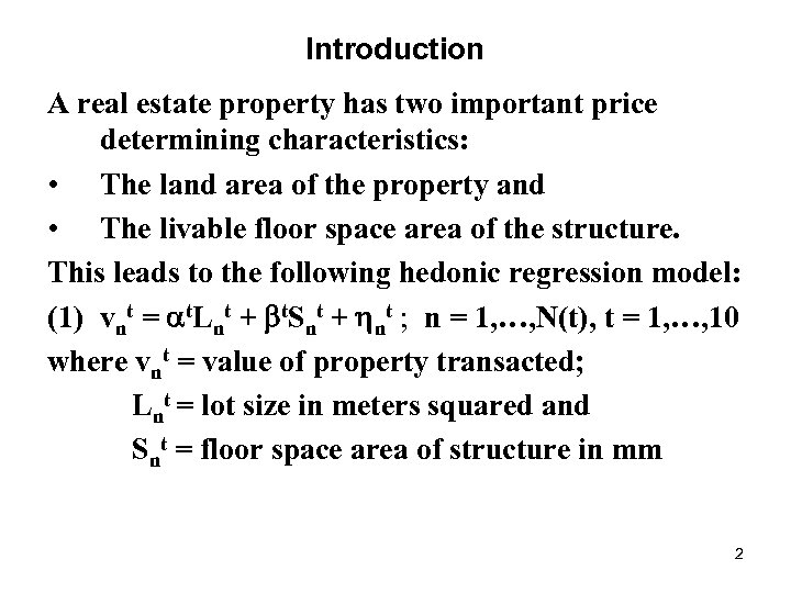 Introduction A real estate property has two important price determining characteristics: • The land area of the property and • The livable floor space area of the structure. This leads to the following hedonic regression model: (1) vnt = t. Lnt + t. Snt + nt ; n = 1, …, N(t), t = 1, …, 10 where vnt = value of property transacted; Lnt = lot size in meters squared and Snt = floor space area of structure in mm 2
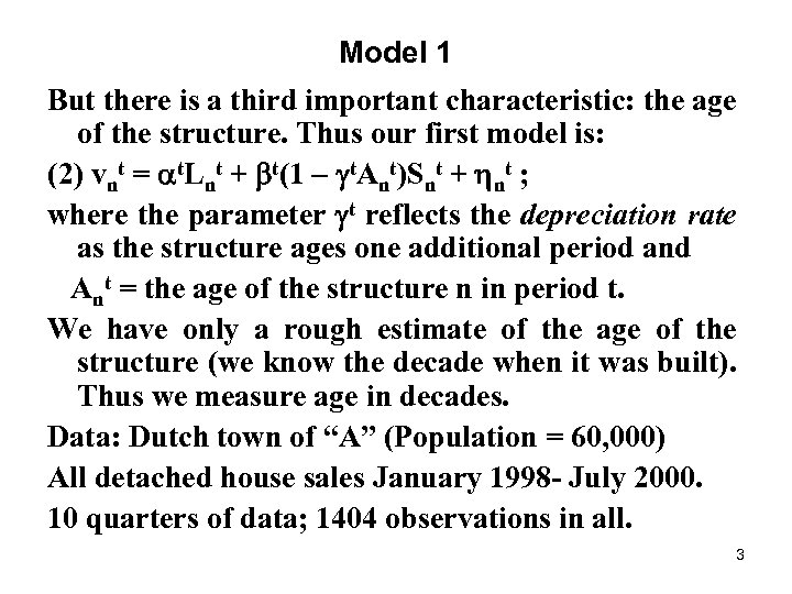 Model 1 But there is a third important characteristic: the age of the structure. Thus our first model is: (2) vnt = t. Lnt + t(1 t. Ant)Snt + nt ; where the parameter t reflects the depreciation rate as the structure ages one additional period and Ant = the age of the structure n in period t. We have only a rough estimate of the age of the structure (we know the decade when it was built). Thus we measure age in decades. Data: Dutch town of “A” (Population = 60, 000) All detached house sales January 1998 - July 2000. 10 quarters of data; 1404 observations in all. 3
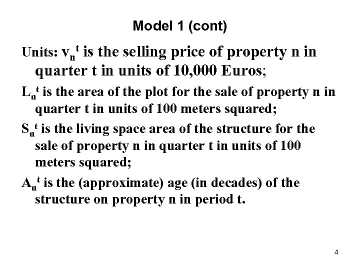 Model 1 (cont) Units: vnt is the selling price of property n in quarter t in units of 10, 000 Euros; Lnt is the area of the plot for the sale of property n in quarter t in units of 100 meters squared; Snt is the living space area of the structure for the sale of property n in quarter t in units of 100 meters squared; Ant is the (approximate) age (in decades) of the structure on property n in period t. 4
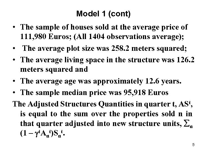 Model 1 (cont) • The sample of houses sold at the average price of 111, 980 Euros; (All 1404 observations average); • The average plot size was 258. 2 meters squared; • The average living space in the structure was 126. 2 meters squared and • The average was approximately 12. 6 years. • The sample median price was 95, 918 Euros The Adjusted Structures Quantities in quarter t, ASt, is equal to the sum over the properties sold n in that quarter adjusted into new structure units, n (1 t. Ant)Snt. 5
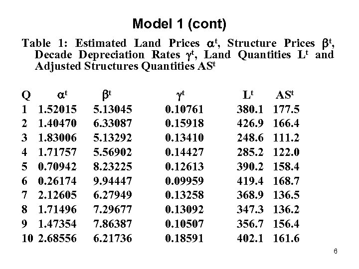 Model 1 (cont) Table 1: Estimated Land Prices t, Structure Prices t, Decade Depreciation Rates t, Land Quantities Lt and Adjusted Structures Quantities ASt Q 1 2 3 4 5 6 7 8 9 10 t 1. 52015 1. 40470 1. 83006 1. 71757 0. 70942 0. 26174 2. 12605 1. 71496 1. 47354 2. 68556 t Lt 5. 13045 0. 10761 380. 1 6. 33087 0. 15918 426. 9 5. 13292 0. 13410 248. 6 5. 56902 0. 14427 285. 2 8. 23225 0. 12613 390. 2 9. 94447 0. 09959 419. 4 6. 27949 0. 13258 368. 9 7. 29677 0. 13092 347. 3 7. 86387 0. 10507 356. 7 6. 21736 0. 18591 402. 1 ASt 177. 5 166. 4 111. 2 122. 0 158. 4 168. 7 136. 5 136. 2 156. 4 161. 6 6
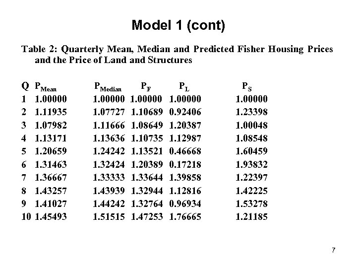 Model 1 (cont) Table 2: Quarterly Mean, Median and Predicted Fisher Housing Prices and the Price of Land Structures Q 1 2 3 4 5 6 7 8 9 10 PMean 1. 00000 1. 11935 1. 07982 1. 13171 1. 20659 1. 31463 1. 36667 1. 43257 1. 41027 1. 45493 PMedian 1. 00000 1. 07727 1. 11666 1. 13636 1. 24242 1. 32424 1. 33333 1. 43939 1. 44242 1. 51515 PF 1. 00000 1. 10689 1. 08649 1. 10735 1. 13521 1. 20389 1. 33644 1. 32944 1. 32764 1. 47253 PL 1. 00000 0. 92406 1. 20387 1. 12987 0. 46668 0. 17218 1. 39858 1. 12816 0. 96934 1. 76665 PS 1. 00000 1. 23398 1. 00048 1. 08548 1. 60459 1. 93832 1. 22397 1. 42225 1. 53278 1. 21185 7
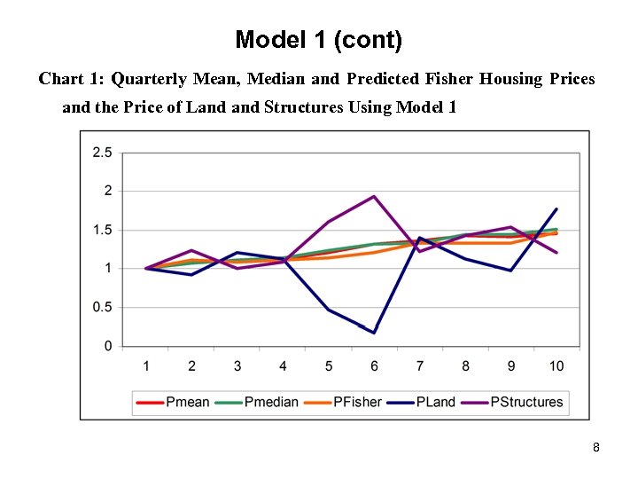 Model 1 (cont) Chart 1: Quarterly Mean, Median and Predicted Fisher Housing Prices and the Price of Land Structures Using Model 1 8
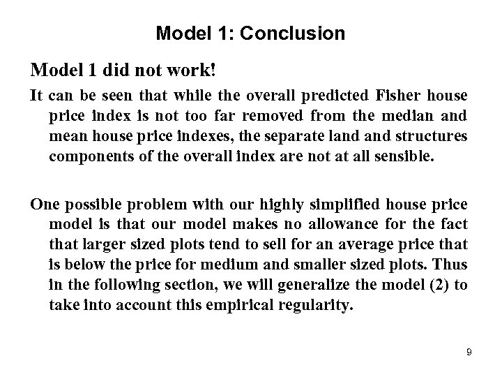 Model 1: Conclusion Model 1 did not work! It can be seen that while the overall predicted Fisher house price index is not too far removed from the median and mean house price indexes, the separate land structures components of the overall index are not at all sensible. One possible problem with our highly simplified house price model is that our model makes no allowance for the fact that larger sized plots tend to sell for an average price that is below the price for medium and smaller sized plots. Thus in the following section, we will generalize the model (2) to take into account this empirical regularity. 9
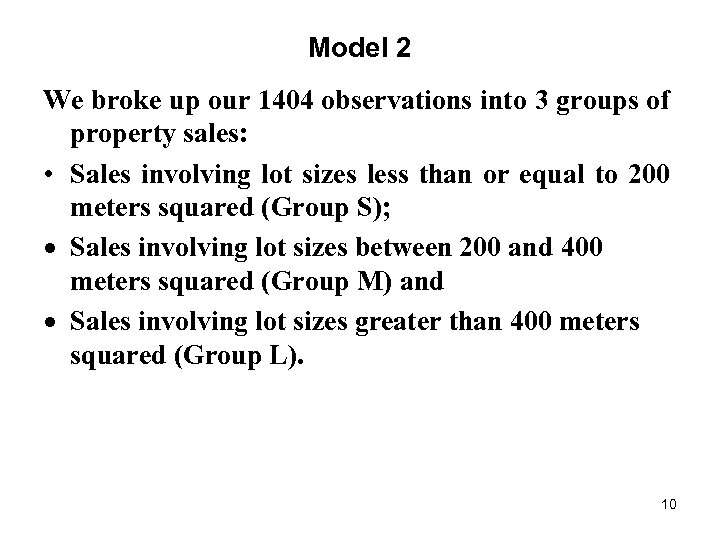 Model 2 We broke up our 1404 observations into 3 groups of property sales: • Sales involving lot sizes less than or equal to 200 meters squared (Group S); · Sales involving lot sizes between 200 and 400 meters squared (Group M) and · Sales involving lot sizes greater than 400 meters squared (Group L). 10
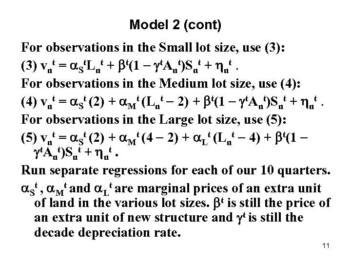 Model 2 (cont) For observations in the Small lot size, use (3): (3) vnt = St. Lnt + t(1 t. Ant)Snt + nt. For observations in the Medium lot size, use (4): (4) vnt = St (2) + Mt (Lnt 2) + t(1 t. Ant)Snt + nt. For observations in the Large lot size, use (5): (5) vnt = St (2) + Mt (4 2) + Lt (Lnt 4) + t(1 t. Ant)Snt + nt. Run separate regressions for each of our 10 quarters. St , Mt and Lt are marginal prices of an extra unit of land in the various lot sizes. t is still the price of an extra unit of new structure and t is still the decade depreciation rate. 11
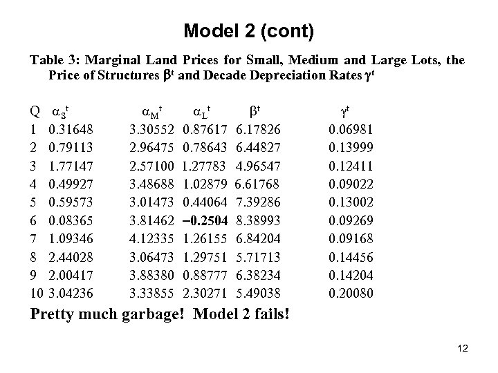 Model 2 (cont) Table 3: Marginal Land Prices for Small, Medium and Large Lots, the Price of Structures t and Decade Depreciation Rates t Q 1 2 3 4 5 6 7 8 9 10 S t 0. 31648 0. 79113 1. 77147 0. 49927 0. 59573 0. 08365 1. 09346 2. 44028 2. 00417 3. 04236 t 3. 30552 2. 96475 2. 57100 3. 48688 3. 01473 3. 81462 4. 12335 3. 06473 3. 88380 3. 33855 L t 0. 87617 0. 78643 1. 27783 1. 02879 0. 44064 0. 2504 1. 26155 1. 29751 0. 88777 2. 30271 t 6. 17826 6. 44827 4. 96547 6. 61768 7. 39286 8. 38993 6. 84204 5. 71713 6. 38234 5. 49038 t 0. 06981 0. 13999 0. 12411 0. 09022 0. 13002 0. 09269 0. 09168 0. 14456 0. 14204 0. 20080 Pretty much garbage! Model 2 fails! 12
 Model 2 (conclusion) Looking at the median price of a house over the 10 quarters in our sample, the median price never fell over the sample period. This fact suggests that we should impose this condition on all of our prices; i. e. , we should set up a nonlinear regression where the marginal prices of land never fall from quarter to quarter and where the price of a square meter of a new structure also never falls. We will do this in the following model and we will also impose a single depreciation rate over our sample period, rather than allowing the depreciation rate to fluctuate from quarter to quarter. 13
 Model 3 The equations that describe the model in quarter 1 are the same as equations (3), (4) and (5) in the previous section except that the quarter one depreciation rate parameter, 1, is replaced by the parameter , which will be used in all subsequent quarters. For the remaining quarters, equations (3), (4) and (5) can still be used except that the parameters St, Mt, Lt and t are set equal to their quarter 1 counterparts plus a sum of squared parameters where one squared parameter is added each period; i. e. , St, Mt, Lt and t are reparameterized as follows: 14
 Model 3 (cont) (6) St = S 1 + ( S 2)2 +. . . + ( St)2 ; (7) Mt = M 1 + ( M 2)2 +. . . + ( Mt)2 ; (8) Lt = L 1 + ( L 2)2 +. . . + ( Lt)2 ; (9) t = 1 + ( 2)2 +. . . + ( t)2 The results of the above model were as follows: the quarter 1 estimated parameters were S 1 = 0. 56040 (0. 24451), M 1 = 3. 4684 (0. 11304), L 1 = 0. 33729 (0. 04310), 1 = 6. 2987 (0. 39094) and = 0. 11512 (0. 006664), (standard errors in brackets) with an R 2 of. 8439. Thus the overall decade depreciation rate was a very reasonable 11. 5%. Surprise: marginal valuation for land for small lots much smaller than for medium lots. As expected, the valuation for large lots was less than for medium lots. 15
 Model 3 (cont) Of the 36 squared parameters that pertain to quarters 2 to 10, 23 were set equal to 0 by the nonlinear regression and only 13 were nonzero with only 8 of these nonzero parameters having t statistics greater than 2. The quarter by quarter values of the parameters St Mt Lt and t defined by (6)-(9) are reported in Table 4 below. Thus we had only 18 nonzero parameters to explain 1404 observations. 16
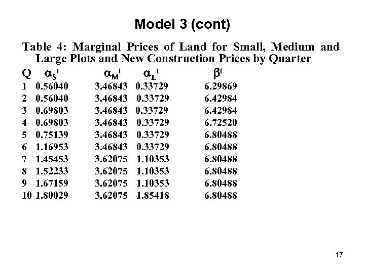 Model 3 (cont) Table 4: Marginal Prices of Land for Small, Medium and Large Plots and New Construction Prices by Quarter Q St t Lt t 1 2 3 4 5 6 7 8 9 10 0. 56040 0. 69803 0. 75139 1. 16953 1. 45453 1. 52233 1. 67159 1. 80029 3. 46843 3. 62075 0. 33729 1. 10353 1. 85418 6. 29869 6. 42984 6. 72520 6. 80488 17
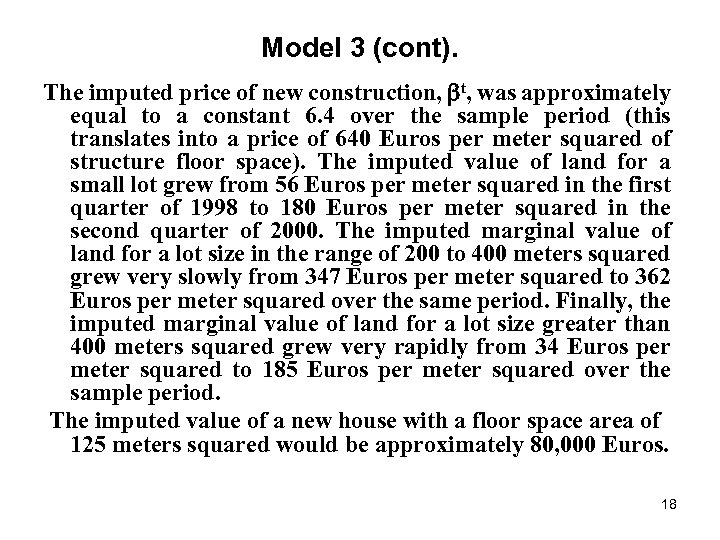 Model 3 (cont). The imputed price of new construction, t, was approximately equal to a constant 6. 4 over the sample period (this translates into a price of 640 Euros per meter squared of structure floor space). The imputed value of land for a small lot grew from 56 Euros per meter squared in the first quarter of 1998 to 180 Euros per meter squared in the second quarter of 2000. The imputed marginal value of land for a lot size in the range of 200 to 400 meters squared grew very slowly from 347 Euros per meter squared to 362 Euros per meter squared over the same period. Finally, the imputed marginal value of land for a lot size greater than 400 meters squared grew very rapidly from 34 Euros per meter squared to 185 Euros per meter squared over the sample period. The imputed value of a new house with a floor space area of 125 meters squared would be approximately 80, 000 Euros. 18
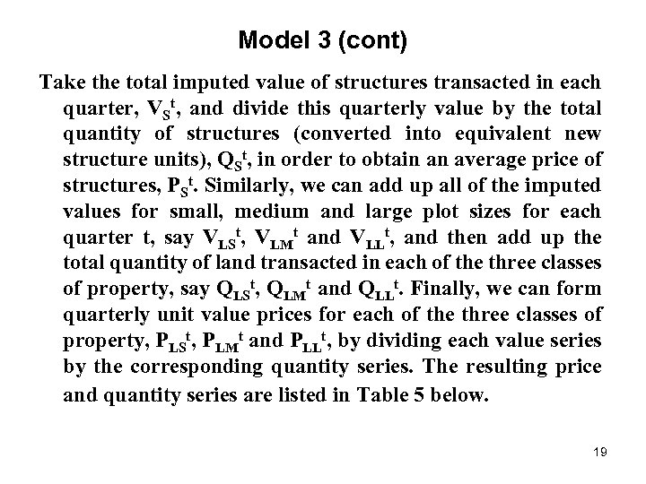 Model 3 (cont) Take the total imputed value of structures transacted in each quarter, VSt, and divide this quarterly value by the total quantity of structures (converted into equivalent new structure units), QSt, in order to obtain an average price of structures, PSt. Similarly, we can add up all of the imputed values for small, medium and large plot sizes for each quarter t, say VLSt, VLMt and VLLt, and then add up the total quantity of land transacted in each of the three classes of property, say QLSt, QLMt and QLLt. Finally, we can form quarterly unit value prices for each of the three classes of property, PLSt, PLMt and PLLt, by dividing each value series by the corresponding quantity series. The resulting price and quantity series are listed in Table 5 below. 19
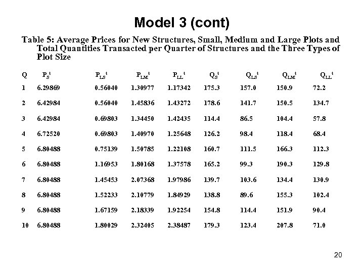 Model 3 (cont) Table 5: Average Prices for New Structures, Small, Medium and Large Plots and Total Quantities Transacted per Quarter of Structures and the Three Types of Plot Size Q PSt 1 6. 29869 2 PLSt PLMt PLLt QSt QLMt QLLt 0. 56040 1. 30977 1. 17342 175. 3 157. 0 150. 9 72. 2 6. 42984 0. 56040 1. 45836 1. 43272 178. 6 141. 7 150. 5 134. 7 3 6. 42984 0. 69803 1. 34450 1. 42435 114. 4 86. 5 104. 4 57. 8 4 6. 72520 0. 69803 1. 40970 1. 25648 126. 2 98. 4 118. 4 68. 4 5 6. 80488 0. 75139 1. 50785 1. 22108 160. 7 111. 5 166. 3 112. 3 6 6. 80488 1. 16953 1. 80168 1. 37578 165. 2 99. 3 190. 3 129. 8 7 6. 80488 1. 45453 2. 07368 1. 97986 139. 7 103. 6 134. 4 130. 9 8 6. 80488 1. 52233 2. 10779 1. 84929 138. 8 89. 6 155. 3 102. 4 9 6. 80488 1. 67159 2. 18339 1. 92254 154. 8 114. 4 151. 9 90. 4 10 6. 80488 1. 80029 2. 32405 2. 38487 179. 3 123. 4 207. 8 71. 0 20
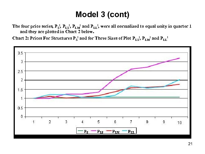 Model 3 (cont) The four price series, PSt, PLMt and PLLt, were all normalized to equal unity in quarter 1 and they are plotted in Chart 2 below. Chart 2: Prices For Structures PSt and for Three Sizes of Plot PLSt, PLMt and PLLt 21
 Model 3 (cont) The data listed in Table 5 were further aggregated. We constructed a chained Fisher aggregate for the three land series and the resulting aggregate land price and quantity series, PLt and QLt, are listed in Table 6 below along with the structures price and quantity series (normalized so that the price equals 1 in quarter 1), PSt and QSt. Finally, a chained Fisher aggregate for structures and the three land series was constructed and the resulting aggregate price and quantity series, Pt and Qt, are also listed in Table 6. 22
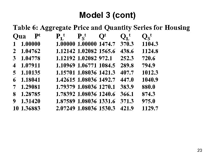 Model 3 (cont) Table 6: Aggregate Price and Quantity Series for Housing Qua Pt PLt P St Qt QLt Q St 1 2 3 4 5 6 7 8 9 10 1. 00000 1. 04762 1. 04778 1. 07911 1. 10135 1. 18041 1. 29081 1. 28785 1. 31420 1. 36883 1. 00000 1. 12142 1. 12192 1. 10969 1. 15701 1. 42615 1. 79379 1. 78392 1. 87589 2. 07249 1. 00000 1. 02082 1. 06771 1. 08036 1474. 7 1565. 6 972. 1 1084. 5 1421. 3 1492. 7 1270. 1 1240. 6 1331. 6 1530. 3 370. 3 438. 6 252. 3 289. 8 407. 7 447. 0 383. 9 366. 1 371. 3 421. 9 1104. 3 1124. 8 720. 6 794. 9 1012. 3 1040. 9 880. 0 874. 3 975. 0 1129. 7 23
 Model 3 (cont) Chart 3: Quarterly Mean Price PMeant, Median Price PMedian, Constant Quality P, Land Price PL and New Structures Price PS 2. 5 2 1. 5 1 0. 5 0 1 2 3 4 PMean 5 PMedian 6 7 P PL 8 9 10 PS 24
 Model 3 (concluded) From Chart 3, it is evident that our estimated constant quality price of housing for City A grew more slowly than the corresponding mean and median series. The major explanatory factor for this difference is due to the fact that the average of the structure tended to fall as time marched on. We also tried log-log and semilog hedonic models but the resulting price series for land structures were not sensible. The semilog model did not fit well. Overall, Model 3 looks promising! We have explained 84% of the price variation using only 3 characteristics and the resulting prices are not crazy! 25
 Conclusion Our tentative conclusion at this point is that hedonic regression techniques can be used in order to decompose the selling prices of properties into their land structure components but it is not a completely straightforward exercise. In particular, monotonicity restrictions on the parameters will generally have to be imposed on the model in order to obtain sensible results. Our results also indicate that stable coefficients cannot be obtained using just data for one quarter. An open question is: how many quarters of data do we need to run in the one big nonlinear regression in order to obtain stable imputed prices for land structures? 26
 Questions for further research • Can our method be adapted to monthly data? · Can we adapt our method into a rolling year method; i. e. , we use only the data for a full year plus one additional time period and use the results to update our previous series? · We did not eliminate any outliers in our preliminary research. Do we get similar results if outliers are eliminated? About 15 -20% of our observations could be classified as outliers; i. e. , the predicted sale price differs from the actual sale price by more than 20, 000 Euros. · Is it worthwhile to consider more characteristics or would it be more efficient to simply eliminate outliers? • How does our suggested method compare to the repeat sales method? 27


