34f3ebe5e686bd7e58b17db8a42931f0.ppt
- Количество слайдов: 48
The Coase Theorem & Game Theory Presented by Dr. Elizabeth Hoffman IRLE May 22, 2006 Professor of Economics and CU President Emerita

Coase Experiment

Coase Experiments Payoff Sheet Number A’s Payoff B’s Payoff 1 $0. 00 $12. 00 2 4. 00 10. 00 3 7. 50 4. 00 4 7. 50 4. 00 5 9. 00 2. 50 6 10. 50 1. 00 7 12. 00 0. 00
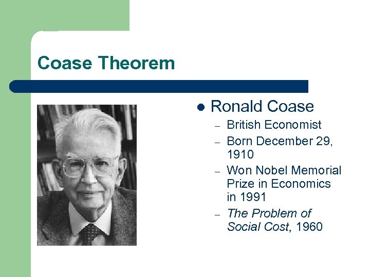
Coase Theorem l Ronald Coase – – British Economist Born December 29, 1910 Won Nobel Memorial Prize in Economics in 1991 The Problem of Social Cost, 1960
Coase Theorem l Owner of property right will manage production or negotiate a price such that those not owning property right will pay l Assign property rights: – To pollute – To breath clean air – To a fishery – To an oil pool
Coase Theorem l Coase argued outcome would be efficient, only the distribution of resources would be affected. l Examples: – Farmer and rancher decide how much land to fence for farming and how much to allow as open range for cattle – Railroad and farmer will decide how close to the tracks to allow crops to grow and how much burning from sparks to allow

Coase Theorem l Experimental Tests of the Coase Theorem – – – Property rights by the flip of a coin Large bargaining groups Property rights by earned entitlement and moral authority

Coase Theorem Experimental Results Number of Decisions (N) Number of Joint Maxima (N 1) Equal Split (N 2) 22 20 10 20 19 9 22 18 9 22 21 4 86 78 32 Experiment A. Coin flip: 1. No moral authority 2. Moral authority B. Game trigger: 1. No moral authority 2. Moral authority Total
Coase Theorem l Problems with the Coase Theorem – – – Assignment of property rights can be disputed in the legal system (tort law) Transaction costs may lead to different outcomes depending on which side has property right Imperfect or asymmetric information about valuations Free rider problem comes into effect when more than one person shares property right Pooling can result in last owner holding out to get all the profits Others, not included in bargaining, may be affected by outcome

Nash Equilibrium l John Nash – – – American Mathematician Born June 13, 1928 Won Nobel Memorial Prize in Economics in 1994 for Game Theory
Cournot-Nash Equilibrium l l l Cournot – 19 th century economist who first came up with an idea to formalize Adam Smith’s theory of perfect competition Games and Economic Behavior by von Neumann and Morgenstern (1944), first real book in game theory Nash developed a simple way to illustrate points made by both Cournot and von Neumann and Morgenstern

Cournot-Nash Equilibrium l Definition: – Assuming players are maximizing in their own interest, each player plays a strategy which optimizes for that player, given what strategies the other players are playing. A Nash equilibrium is a set of strategies, such that when every one is maximizing, given all other players’ strategies, no player has an incentive to change his or her strategy.
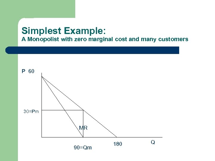
Simplest Example: A Monopolist with zero marginal cost and many customers P 60 30=Pm MR 90=Qm 180 Q
Simplest Example: A Monopolist with zero marginal cost and many customers The demand curve intersects the quantity axis at 180 units. Therefore, the marginal revenue curve intersects the quantity axis at ½ of 180, or 90. The monopolist maximizes profits by equating a marginal cost of 0 and a marginal revenue of 0, producing 90 units and charging a price that sells 90 units. Since there are many consumers, no one consumer can affect the market by unilaterally changing his or her behavior. Thus, the monopolist’s decision is a Nash equilibrium.
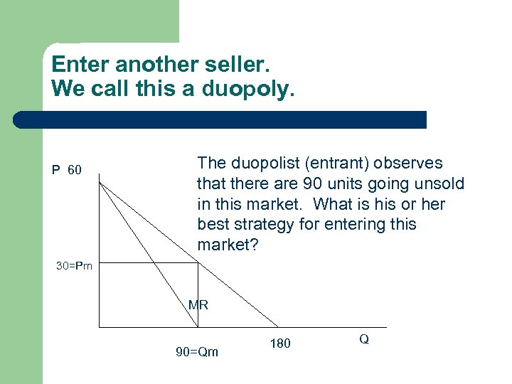
Enter another seller. We call this a duopoly. P 60 The duopolist (entrant) observes that there are 90 units going unsold in this market. What is his or her best strategy for entering this market? 30=Pm MR 90=Qm 180 Q
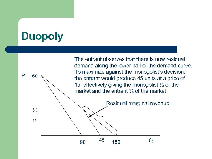
Duopoly P 60 The entrant observes that there is now residual demand along the lower half of the demand curve. To maximize against the monopolist’s decision, the entrant would produce 45 units at a price of 15, effectively giving the monopolist ½ of the market and the entrant ¼ of the market. Residual marginal revenue 30 15 90 45 180 Q
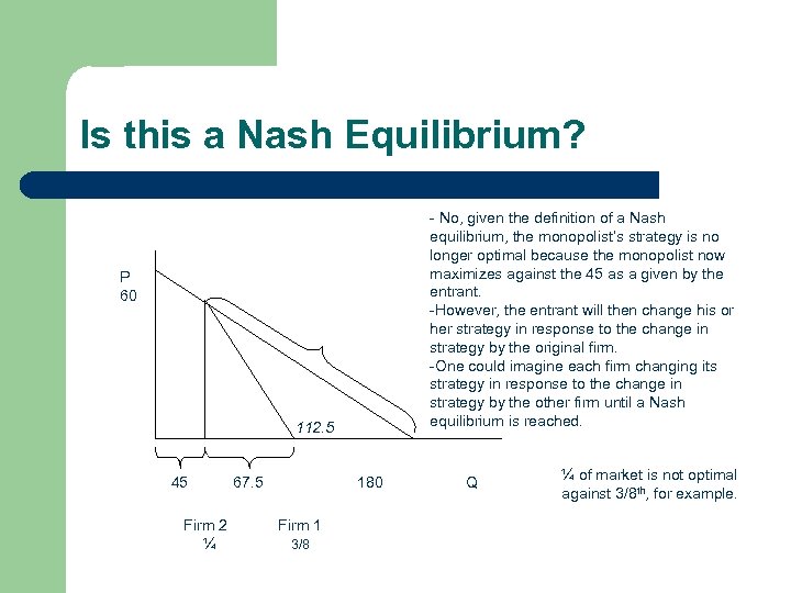
Is this a Nash Equilibrium? - No, given the definition of a Nash equilibrium, the monopolist’s strategy is no longer optimal because the monopolist now maximizes against the 45 as a given by the entrant. -However, the entrant will then change his or her strategy in response to the change in strategy by the original firm. -One could imagine each firm changing its strategy in response to the change in strategy by the other firm until a Nash equilibrium is reached. P 60 112. 5 45 Firm 2 ¼ 67. 5 180 Firm 1 3/8 Q ¼ of market is not optimal against 3/8 th, for example.
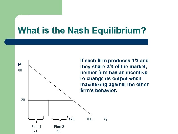
What is the Nash Equilibrium? If each firm produces 1/3 and they share 2/3 of the market, neither firm has an incentive to change its output when maximizing against the other firm’s behavior. P 60 20 120 Firm 1 60 Firm 2 60 180 Q
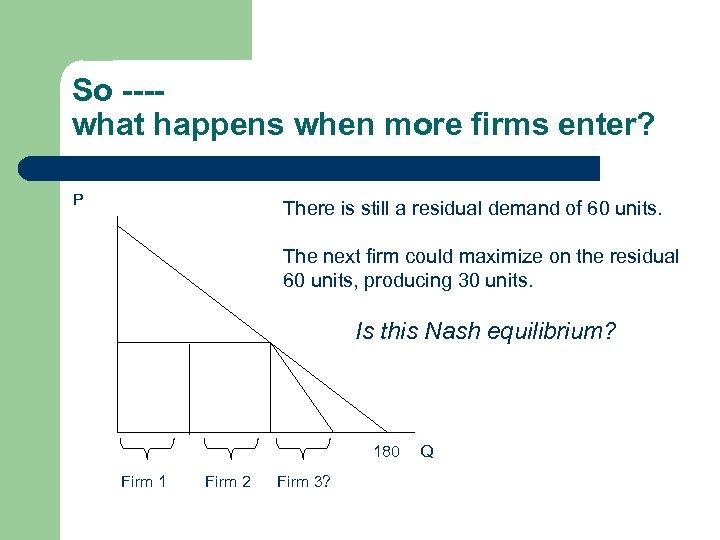
So ---what happens when more firms enter? P There is still a residual demand of 60 units. The next firm could maximize on the residual 60 units, producing 30 units. Is this Nash equilibrium? 180 Firm 1 Firm 2 Firm 3? Q
Nash Equilibrium Previous slide NOT Nash Equilibrium because other firms would once again respond. What would be Nash equilibrium? Divide in ¼’ths?
Nash Equilibrium Suppose a thousand firms enter? Suppose there an infinite number of firms? – – Quantity produced goes to 180, price goes to zero. Obviously, if there is a positive marginal cost, quantity will be driven to the quantity that equates marginal cost and marginal revenue. Therefore, the simplest Nash equilibrium with many firms and many consumers is a competitive equilibrium!
So, what is a game in economics? l A set of players (firms, consumers, governments), a set of alternative strategies available to each player, and a set of payoffs obtainable as a function of the strategies simultaneously played by all the players.

Cooperative and non-cooperative games: A non-zero sum game is a game in which there exists a joint-profit maximum if the players can agree to play the game as a cooperative game. Thus, the monopoly game described above could be played as a cooperative game if the players could agree to split the monopoly profits and restrict output to the monopoly output.

Cooperative and non-cooperative games: When a group of firms succeeds in colluding we call it a cartel. OPEC is such a cartel. Cartels were rendered illegal in the U. S. in 1890 under the Sherman Anti-trust Act after the railroad consolidations and John D. Rockefeller’s Standard Oil Trust.
Cooperative and non-cooperative games: A zero-sum game is a game in which one player’s gain is always another player’s loss. Zero-sum games can only be played as noncooperative games, since there exists no joint maximizing solution.

Core: l The core of a cooperative game is a solution that maximizes the joint profits and guarantees each player at least as much as he or she could earn alone or by cooperating with any smaller group among the other firms. We call any smaller group a coalition.
Back to the Coase Theorem Experiments
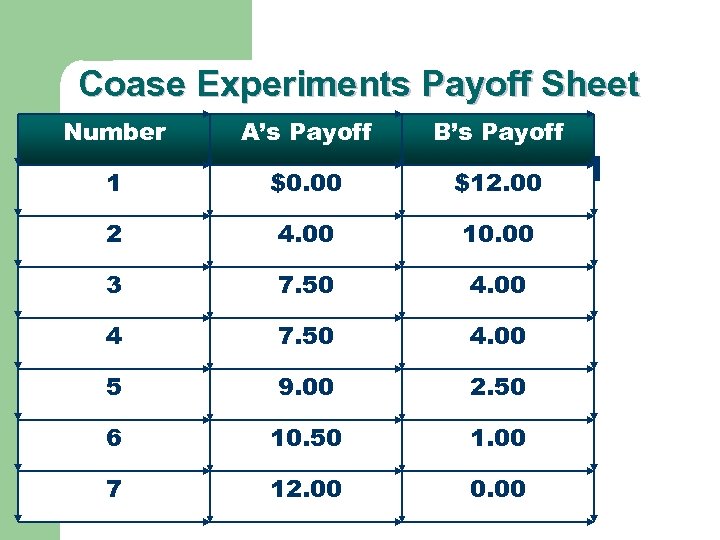
Coase Experiments Payoff Sheet Number A’s Payoff B’s Payoff 1 $0. 00 $12. 00 2 4. 00 10. 00 3 7. 50 4. 00 4 7. 50 4. 00 5 9. 00 2. 50 6 10. 50 1. 00 7 12. 00 0. 00

What is the Core and why? – – Number 2 maximizes the joint profits but the controller has to earn at least $12 to be as well off as if he or she played the game as a noncooperative game. If the players were to divide the $2 of surplus, equally, we would call it a Nash bargaining solution.
Thus, the Nash equilibrium of the Coase game is to take the $12 and run, the core is to agree to outcome 2, and give the controller at least $12, and the Nash bargaining solution is to agree to outcome 2 and split the $2.
The Prisoner’s Dilemma: Another example of a non-zero sum game that can be played cooperatively or non-cooperatively In the prisoner’s dilemma, there are two suspects accused of a crime. They are separated in two rooms and grilled. If they stick together and don’t confess, each might get off or get off lightly. Each is offered a chance to rat on the other in return for no conviction and a big conviction for the other person. If both rat, they both get sentences, perhaps not quite as bad as if only one rats.
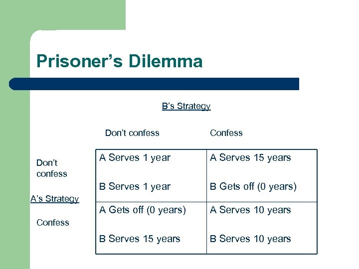
Prisoner’s Dilemma B’s Strategy Don’t confess Confess A Serves 1 year A Serves 15 years B Serves 1 year B Gets off (0 years) A Gets off (0 years) Don’t confess A Serves 10 years B Serves 15 years B Serves 10 years A’s Strategy Confess
Prisoner’s Dilemma What is the Nash equilibrium strategy? For prisoner A, if B doesn’t confess, he should confess, because he gets off. Similarly, for prisoner B, if A doesn’t confess, he should confess, because he gets off. Thus, both confess and get 10 years. We call this a dominant strategy Nash equilibrium or a strong Nash equilibrium because no other strategy dominates unless they succeed in sticking together and actively colluding.
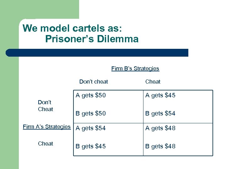
We model cartels as: Prisoner’s Dilemma Firm B’s Strategies Don’t cheat Cheat A gets $50 A gets $45 B gets $50 B gets $54 Firm A’s Strategies A gets $54 A gets $48 Don’t Cheat B gets $45 B gets $48
We model cartels as: Prisoner’s Dilemma The joint profit maximum is not to cheat and split $100. But each has a dominant strategy to cheat for the extra $4. The end result is that they split $96, leaving $4 on the table.
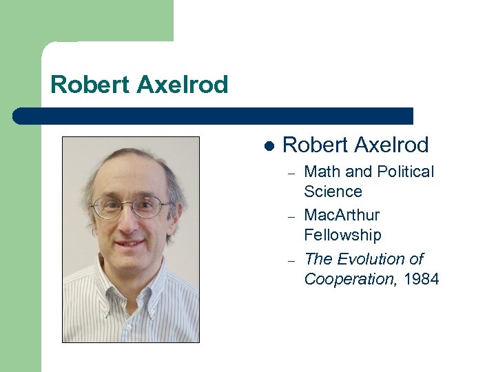
Robert Axelrod l Robert Axelrod – – – Math and Political Science Mac. Arthur Fellowship The Evolution of Cooperation, 1984
Robert Axelrod, The Evolution of Cooperation, (1984) studied the Prisoner’s Dilemma when played by the same two players repeatedly for many periods. He formalized the type of strategic interaction that would occur when the Prisoner’s Dilemma is played repeatedly. In tit-for-tat, player 1 starts by cooperating and then each player simply repeats what the other player does.
Robert Axelrod came up with this idea after running an iterated prisoner’s game contest, in which game theorists were invited to submit computer programs for how to play an iterated prisoner’s dilemma game against all other strategies. Anatol Rapaport submitted the winning strategy, a four-line program, which became known as tit-for-tat. Sometimes it is played with “forgiveness”.
Robert Axelrod l l Later, a team from Southampton University (Nicholas Jennings, Rejdeep Dash, Sarvapali Rachurn, Alex Rogers, and Perukrishnen Vytelingum) introduced a more complicated, more forgiving tit-for-tat strategy that beat Rapaport’s. But, if it encounters a constant defector, it always defects. What this leads to is an understanding that social norms of behavior have powerful effect on how people actually play economic games in the real world.
Robert Axelrod l l Social norms favoring cooperation have powerful evolutionary bases because our species would not have survived the trials of living in the African grasslands if we had not learned to cooperate effectively and to punish cheaters swiftly and effectively. This brings us to work by Hoffman, Mc. Cabe, and Smith on the ultimatum game.
Ultimatum Game Experiment
Ultimatum Game Experiment l l In the ultimatum game, there are two players who must split a sum of money. One makes a proposal. The other must agree or disagree. If the second agrees, the division takes place. If the second disagrees, they get nothing. The smallest offer is $1. What is the Nash equilibrium and why? In the dictator game, the first mover proposes a division. The second mover has no recourse. What is the Nash equilibrium and why?
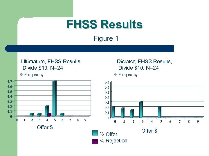
FHSS Results Figure 1 Ultimatum; FHSS Results, Divide $10, N=24 % Frequency Dictator; FHSS Results, Divide $10, N=24 % Frequency Offer $ % Offer % Rejection Offer $
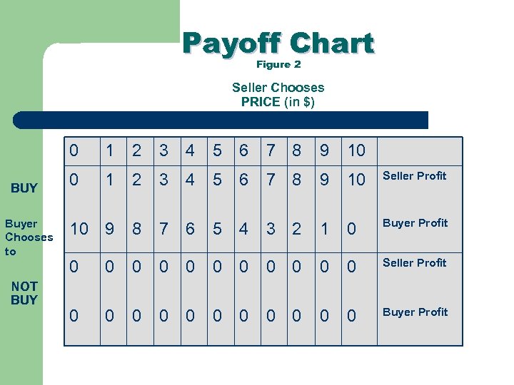
Payoff Chart Figure 2 Seller Chooses PRICE (in $) 0 BUY Buyer Chooses to NOT BUY 1 2 3 4 5 6 7 8 9 10 0 1 2 3 4 5 6 7 8 9 10 Seller Profit 10 9 8 7 6 5 4 3 2 1 0 Buyer Profit 0 0 0 Seller Profit 0 0 0 Buyer Profit

Figure 3 % Offer % Rejection Ultimatum; Contest Entitlement, FHSS Instructions, Divide $10, N=24 % Frequency Ultimatum; Random Entitlement, FHSS Instructions, Divide $10, N=24 Offer $ Ultimatum; Contest Entitlement, Exchange, Divide $10, N=24 % Frequency Ultimatum; Random Entitlement, Exchange, Divide $10, N=24 Offer $

Figure 4 % Offer % Rejection Ultimatum; Contest Entitlement, Exchange, $10, N=24 % Frequency Ultimatum; Random Entitlement, FHSS Instructions, Divide $10, N=24 Offer $ Ultimatum; Contest Entitlement, Exchange, $100, N=23 % Frequency Ultimatum; Random Entitlement, FHSS Instructions, Divide $100, N=27 Offer $
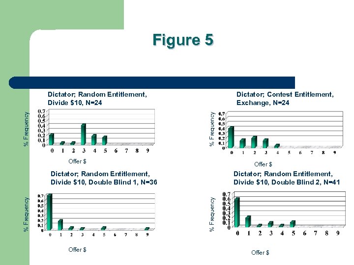
Figure 5 Dictator; Contest Entitlement, Exchange, N=24 % Frequency Dictator; Random Entitlement, Divide $10, N=24 Offer $ Dictator; Random Entitlement, Divide $10, Double Blind 2, N=41 % Frequency Dictator; Random Entitlement, Divide $10, Double Blind 1, N=36 Offer $
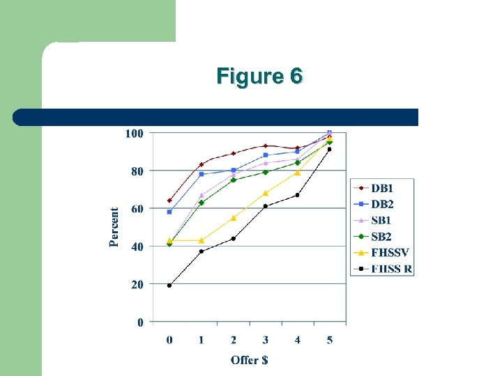
Figure 6
34f3ebe5e686bd7e58b17db8a42931f0.ppt