The Causes of Variation Lindon Eaves and Tim

The Causes of Variation Lindon Eaves and Tim York Boulder, CO March 2001

One Issue (Among Many!) • Identifying genes that cause complex diseases and genes that contribute to variation in quantitative traits

Quantitative Trait Locus (QTL) Any gene whose contribution to variation in a quantitative trait is large enough to stand out against the background noise of other genetic and environmental factors

Quantitative Trait A continuously variable trait (in which variation may be caused by multiple genetic and/or environmental factors); any categorical trait in which differences between categories may be mapped onto variation in a continuous trait

Common diseases • • • Estimated life time risk c. 60% Substantial genetic component “Non-Mendelian” inheritance Non-genetic risk factors Multiple interacting pathways Most genes still not mapped

Examples • • Ischaemic heart disease (30 -50%, F-M) Breast cancer (12%, F) Colorectal cancer (5%) Recurrent major depression (10%) ADHD (5%) Non-insulin dependent diabetes (5%) Essential hypertension (10 -25%)

Even for “simple” diseases: Number of alleles is large (Wright et al, 1999) • Ischaemic heart disease (LDR) >190 • Breast cancer (BRAC 1) >300 • Colorectal cancer (MLN 1) >140

Definitions • Locus: One of c. 30 -40, 000 genes • Allele: One of several variants of a specific gene • Gene: a sequence of DNA that codes for a specific function • Base pair: chemical “letter” of the genome (a gene has many 1000’s of base pairs) • Genome: all the genes considered together

Finding QTLs • Linkage • Association

Linkage Finds QTLs by correlating phenotypic similarity with genetic similarity (“IBD”) in specific parts of genome

Linkage • Doesn’t depend on “guessing gene” • Works over broad regions (good for getting in right ball-park) and whole genome (“genome scan”) • Only detects large effects (>10%) • Requires large samples (10, 000’s? ) • Can’t guarantee close to gene

Association • Looks for correlation between specific alleles and phenotype (trait value, disease risk)

Association • More sensitive to small effects • Need to “guess” gene/alleles (“candidate gene”) or be close enough for linkage disequilibrium with nearby loci • May get spurious association (“stratification”) – need to have genetic controls to be convinced

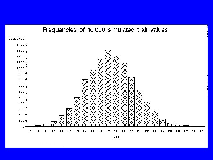
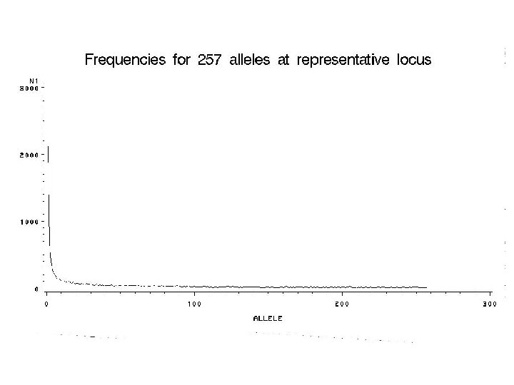
“Reality”: For complex disorders and quantitative traits Large number of alleles at large number of genes

Defining the Haystack • 3 x 109 base pairs • Markers every 6 -10 kb for association in populations with no recent bottleneck history • 1 SNPs per 721 b. p. (Wang et al. , 1998) • c. 14 SNPs per 10 kb = 1000 s haplotypes/alleles • O (104 -105) genes

Problems • Large number of loci and alleles/haplotypes • Possible interactions between genes and environment • Relatively low frequencies of individual risk factors • Functional form of genotype-phenotype relations not known • Sorting out signal from noise – minimizing errors within budget • Scaling of phenotype (continuous, discontinuous) • Spurious association (stratification)

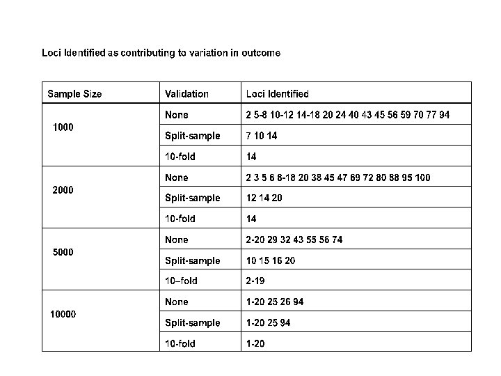
Prepare for the worst Need statistical approaches that can screen enormous numbers of loci and alleles to identify reliably those that have impact on risk to disease

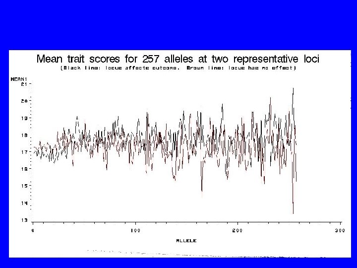
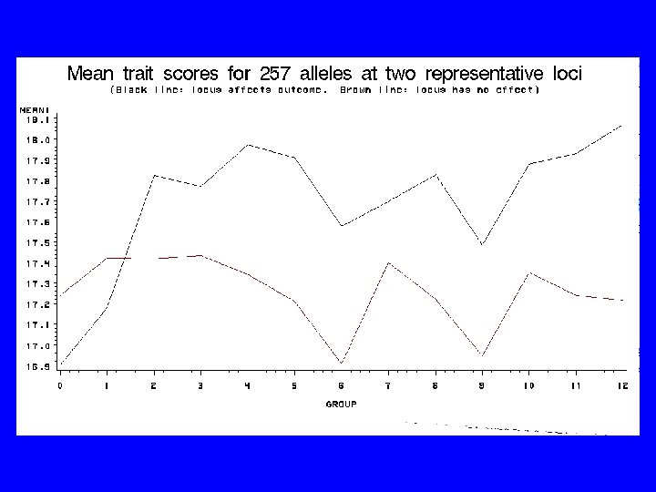
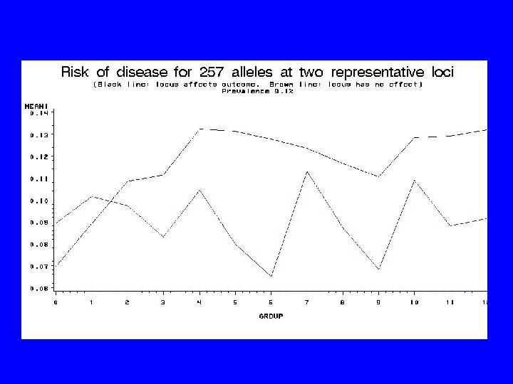
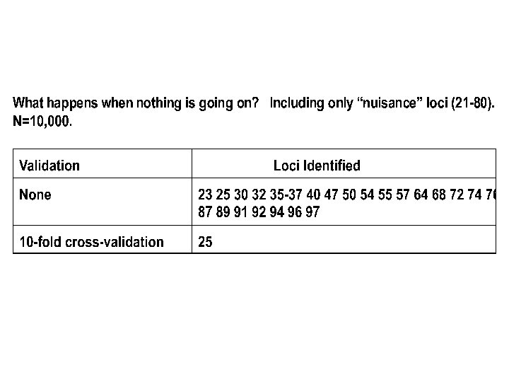
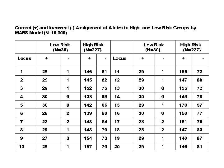
System Chosen for Study • • • 100 loci 20 loci affect outcome, 80 “nuisance” genes 257 alleles/locus Allele frequencies c. 20 -0. 1% Disease genes each explain 2. 5% variance in risk (c. 2 -fold risk increase) • 40% rarest alleles increase risk • 50% variance non-genetic

It’s a Mess! • Don’t know which genes – might have clues • Don’t know which alleles – unordered categories • >250100 locus/allele combinations • More predictor combinations than people (“curse of dimensionality”) • Reality worse

Problems • Informatics: large volume of data • Computational: large number of combinations • Statistical: large number of chance associations • Genetic-epidemiological: secondary associations

How are we going to figure it out?

Data Mining (Steinberg and Cartel) • Attempt to discover possibly very complex structure in huge databases (large number of records and large number of variables) • Problems include classification, regression, clustering, association (market analysis) • Need tools to partially or fully automate the discovery process • Large databases support search for rare but important patterns and interactions (epistasis, Gx. E)

Some Approaches to DM • • Logistic regression Neural networks “CART” (Breiman et al. 1984) “MARS” (Friedman, 1991)

“MARS” • • Multivariate Adaptive Regression Splines

Key references Friedman, J. H. (1991) Multivariate Adaptive Regression Splines (with discussion), Annals of Statistics, 19: 1 -141. Steinberg, D. , Bernstein, B. , Colla, P. , Martin, K. , Friedman, J. H. (1999) MARS User Guide. San Diego, CA: Salford Systems

The MARS Advantage • Allows large number of predictors (loci/alleles/environments) to be screened • Non-parametric • Continuous and discontinuous outcomes • Systematic search for detailed interactions • Testing and cross-validation • Continuous and categorical predictors • Decides best form of relationship

Example Regression Spline: Impact of Non-Retail Business on Median Boston House Prices Median House Price “Knot” Industrial Business

Fitting functions with Splines • Piece-wise linear regression. – simplest form. allow regression to bend. • “Knots” define where the function changes behavior. • Local fit vs. Global fit. actual data spline with 3 knots

One predictor example True knots at 20 and 45 (left) Best single knot at about 35 (right) Y Y 10 20 30 X 40 50 60

10 10 20 20 30 30 40 40 50 50 60 60 10 20 30 40 50 60

Re-express variables as basis functions • Done to generalize the search for knots. Difficult to illustrate splines with > one dimension. • Core building block of MARS model – max (0, X – c); – example: BF 1 = max(0, ENV – 5); BF 2 = max(0, ENV – 8); 0 for ENV <= 5; 1 for 5 <= ENV <= 8; 1 + 2 for ENV > 8; • Weighted sum of basis functions used to approximate the global function. – ie y = constant + 1 * BF 1 + 2 * BF 2 + error;

“Adaptive” Spline • “Optimal” placement of knots • “Optimal” selection of predictors and interactions

Adaptive splines • Problem: – What is the optimal location of knots? – How many knots do you need? – Best to test all variable / knot locations, but computationally burdensome. • MARS solution: – Develop an overfit model with too many knots. – Remove all knots that contribute little to model quality. – The final model should have approximately correct knot locations.

“Optimal” Explains “salient” features of data Ignores irrelevant features Stands up to replication - Several ways to operationalize mathematically

MARS 2 -step model building • Step 1. Growing phase: – begins with only a constant in the model. – serially adds basis functions to a user defined limit. tests each for improvement when added to the model. – addition of basis functions until an overly large model is found. (theoretically the true model is captured). • Step 2. Pruning phase: – delete basis function that contributes least to model fit. – refit the model and delete next term, repeat. – the most parsimonious model is selected. • GCV criterion to select optimal model (Craven 1979). • MARS option uses 10 fold cross-validation to estimate DF.

Cross-validation • Protects against over fitting data. • Develops a model on subset of data. Tests fit on remaining set. • Systematically assesses how many DF to charge each variable entered into model. – Adding a basis function will always lower MSE. – This reduction is penalized by DF charged. • Only backwards deletion step is penalized.

Genetic Example: Regression spline for multi-allelic locus

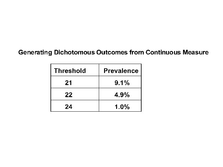
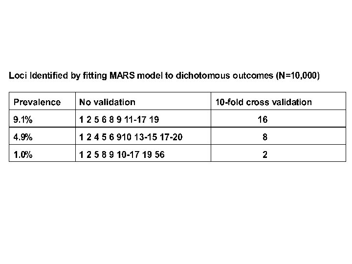
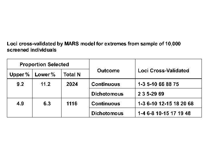
So Far: Does quite well for largish random samples and continuous outcomes. -What about disease (dichotomous) outcomes? -What about selected (extreme) samples?

So? • Can detect signal due to relatively large numbers of relatively rare unordered alleles of relatively small effect at relatively many loci amid the noise of still more loci and environmental effects • “MARS” may provide elements for analyzing such data in this and similar contexts (? microarrays, SNPs, expression arrays? ) • Works with continuous data on random samples and dichotomous outcomes on selected samples

GAW 12 – Simulated data • Provided for two populations: – large general pop. – pop. isolate – founded 20 generations ago by 100 ind. – limited migration b/w. • Common disease: – prevalence of 25%. increases with age – middle age disease, some early onset – more common in females than males

• General population – 7 genes simulated – 13 to 20 kb – 12 to 40 diallelic sites at start of simulation – passed through 120 to 200 K of random mating: • mutation, intragenic recombination, gene conversion – allowed at diff. rates for diff. genes • each gene contains a 500 bp recombination hotspot – 15 to 65% of intragenic recombinations • 8 to 13 mutational hotspots per gene (6 – 300 x’s ) – 25% of genes isolated for 35 to 85 K generations.

GENE 1 GENE 5 Length (kb) 20 17 Start # of SNP 40 20 150 K 165 K . 01 . 002 4 x 10 -8 6 x 10 -9 . 01 . 002 1000 1600 10349 / 50% 4197 / 65% # mutat. hotspot 13 8 Incr mut rate 200 20 Random Mating Rec. rate Mutation rate Gene conv. Mean length conv. Start of rec. hotspot / % in

• Isolate population – loosely modeled after pop. history of Old Order Amish in Lancaster Co. , PA – Founders: 200 chr. ’s sampled from general pop. – 20, 000 chr. ’s sampled from general pop. to create an “outside pop” – Isolate: children <12, mean 4 ; Outside: children <12, 1 – migration allowed b/w pop. s at each generation • rate: migrants = 5% of current isolate size – evolution progressed for 20 generations with recombination (no mutations, no intragenic rec. ) – founders were then sampled to create the isolate pop.

• 23 extended pedigrees with 1, 497 individuals from each population. (1, 000 living) • Pedigrees include the proband, spouse, and all first, second, and third degree relatives of each. • Living individuals are provided: – – – affected status, fid, mid, sex age at last exam age of onset if affected 5 quantitative risk factors 2 environmental risk factors (binary and quantitative) marker genotype for 1 c. M whole genome screen. 2, 855 total markers with an average of 9. 1 alleles – sequence data for 7 candidate genes – 1, 176 sequence variants • 50 replicates provided for each pop.

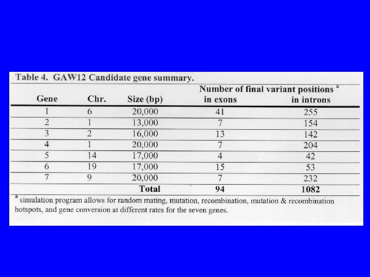
Sequence data • Isolate and General population • Intron and Exon sequence from 7 candidate genes. • Kept only those individuals with sequence data. Each set contain 7, 000 individuals. 64 mb MARS limit. • 5 sets of 7 randomly selected replicates (used 35 of 50 replicates provided) • 5 associated quantitative risk factors. • Covariates included: E 1, E 2, Age, Sex, Age of onset.

• Affected status binary. • Exon sequence coded for each individual as having 0, 1, or 2 ancestral variants. • If intron variant present (whether 1 or 2 copies) given a value of 1. Coded in binary form as haplotypes of length four.

Aff Status E 1 Q 1 MG 1 CG 6 Age of onset MG 6 Liability Q 2 MG 2 Q 3 MG 3 Q 4 E 2 MG 4 CG 1 Q 5 Age MG 5 CG 2

True Model Isolate pop. AFF E 1, Q 1 -Q 5, MG 6 [557] E 1, Q 1 -Q 5, MG 6 [(435 547 548 557) [(27 57 76 110)(435 5244 5268 6912 7281] 547 548 557)] Q 1 E 1, MG 1 [5782] MG 1 [5007] MG 1 [5782] Q 2 E 1, MG 1 [5782] E 1, MG 1 [5007] E 1, MG 1 [5782] Q 3 E 1, E 2 Q 4 E 1, AGE Q 5 E 1, MG 5 [multi-allelic] E 1, MG 5 [1289 3745 8657 8817] ONSET MG 6 [557] none MG 6 [15625] General pop.

Conclusions • MARS works well to capture functional form of disease etiology in simulated data with dichotomous outcome. • In most cases was within 1 Kb of functional variant. • Generated a predictive model that was replicable in at least 4 of 5 data sets. • Highly interpretable output in the form of basis functions and Importance values. • MARS may have problems with highly correlated variables. • Pattern-recognition tools can be useful to narrow down search for genes.

Comparison of MARS and ANN MARS ANN Both are non-parametric estimation schemes, allow for a high number of input predictors, allow for interactions, & non-linear mappings. Maximum allowable basis functions and degree of interactions. Type of network architecture needs to be specified. Models are developed fast. Models are trained more slowly (De. Veaux et al. 1993). Backwards elimination stage to remove Problem of overfitting the data esp. unnecessary basis functions. with small data sets. Easily interpretable basis functions. Local interpretation of the function. Black box-weights have little meaning. Diff. to interpret predictor contribution Penalizes model complexity. Tries to dev. a low order, interpretable model. Non-linear transformations and high connectivity allows for complexity.

But the Haystack is Very Large • • • Reality worse than simulations More alleles at more loci Phenotypes more complex (multivariate) More irrelevant loci (? 1000’s) Interactions with environment and between loci • Spurious associations

It Needs Collaboration Clinical Statistical Molecular Epidemiological Physiological Developmental Informational Evolutionary