The AD-AS Model Lecture 14 academic year

The AD-AS Model Lecture 14 – academic year 2013/14 Introduction to Economics Fabio Landini

Where we are… • Lectures 1 -7: Microeconomics • Lecture 8 -9: GDP, Inflation and unemployment • Lecture 11: Goods market • Lecture 13: Financial market • Lecture 14: Labour market

Questions of the day… • How do we describe the functioning of the economy in the medium period? • Which are the features of the equilibrium in the medium period? • What differentiates the medium period equilibrium from the short period one?

What do we do today? • Premise: short vs. medium period • Construction of the AS curve • Construction of the AD curve • Equilibrium in the short and medium period

Premise: short vs. medium period In Lecture 9 we distinguished three different time horizons: short, medium and long period What differentiates short and medium period? 1) Degree of price flexibility • Short period -> prices are partially flexible • Medium (and long) period -> prices are fully flexible Flexible prices -> Price adjustment mechanism

Premise: short vs. medium period 2) Accuracy of expectations In lecture 14 we introduced the workers’ price expectations (WS curve) In which context are expectations accurate? It is plausible to assume that : • In the short period workers can make errors in forecasting prices (PE can differ from P) • As time passes workers can realize the error and adjust their expectations • In the medium period expectations are assumed to be correct (PE = P)

Premise: short vs. medium period Passage from short to the medium period: Equilibrium in the goods market + Equilibrium in the financial markets + Equilibrium in the labour market AD-AS Model: • Aggregate Supply -> AS • Aggregate Demand -> AD

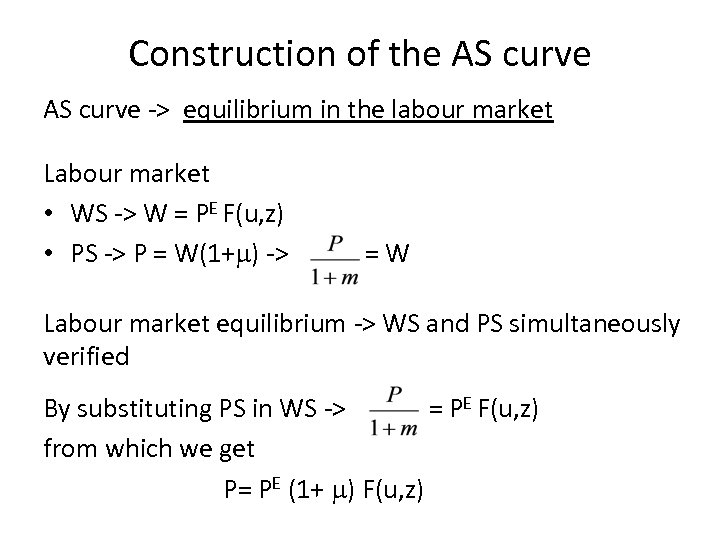Construction of the AS curve -> equilibrium in the labour market Labour market • WS -> W = PE F(u, z) • PS -> P = W(1+m) -> =W Labour market equilibrium -> WS and PS simultaneously verified By substituting PS in WS -> = PE F(u, z) from which we get P= PE (1+ m) F(u, z)

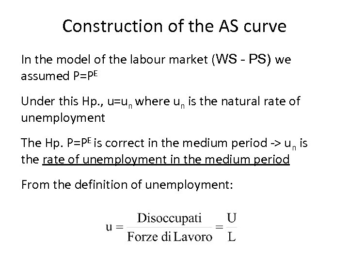Construction of the AS curve In the model of the labour market (WS – PS) we assumed P=PE Under this Hp. , u=un where un is the natural rate of unemployment The Hp. P=PE is correct in the medium period -> un is the rate of unemployment in the medium period From the definition of unemployment:

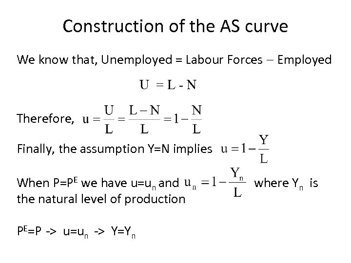Construction of the AS curve We know that, Unemployed = Labour Forces - Employed U =L-N Therefore, Finally, the assumption Y=N implies When P=PE we have u=un and the natural level of production PE=P -> u=un -> Y=Yn where Yn is

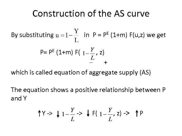Construction of the AS curve By substituting in P = PE (1+m) F(u, z) we get P= PE (1+m) F( , z) + which is called equation of aggregate supply (AS) The equation shows a positive relationship between P and Y Y -> -> F( , z) -> P

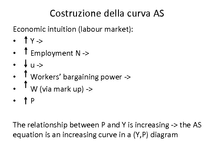Costruzione della curva AS Economic intuition (labour market): • Y -> • Employment N -> • u -> • Workers’ bargaining power -> • W (via mark up) -> • P The relationship between P and Y is increasing -> the AS equation is an increasing curve in a (Y, P) diagram

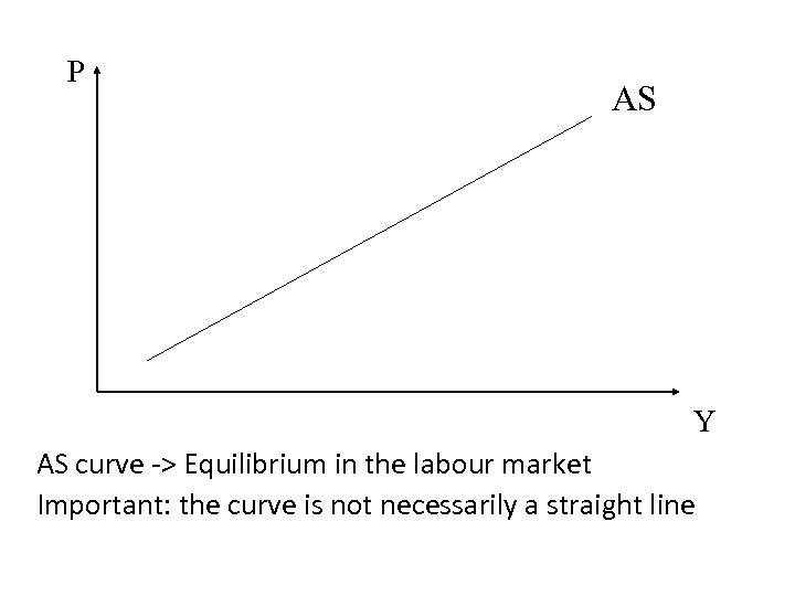P AS Y AS curve -> Equilibrium in the labour market Important: the curve is not necessarily a straight line

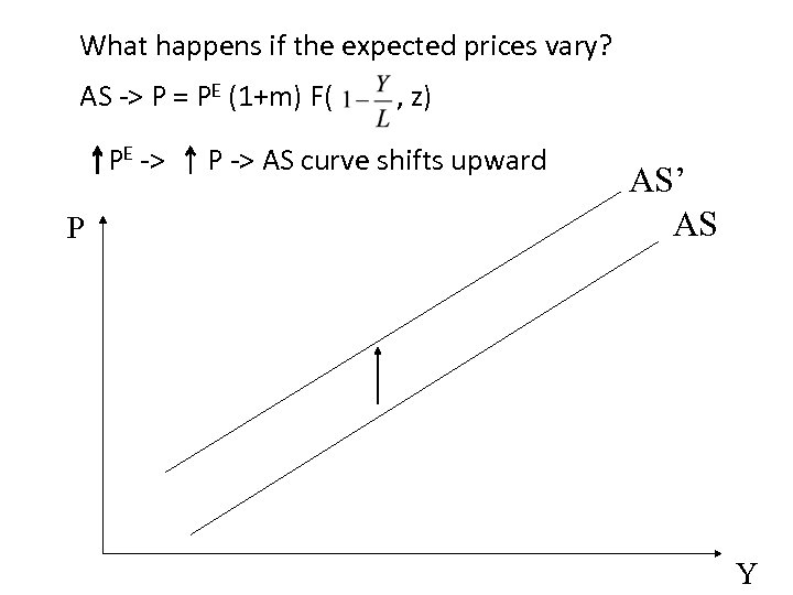What happens if the expected prices vary? AS -> P = PE (1+m) F( PE -> P , z) P -> AS curve shifts upward AS’ AS Y

Construction of the AD curve In constructing the AD curve let’s first consider the goods market and the financial markets in isolation While deriving the aggregate demand (goods market Lecture 11) we assumed that investments were exogenous (I=I 0). Let’s now try to make investments endogenous What do firms consider when they have to decide how much to invest? Mainly two things: 1) Sales. If I sell more I need to produce more -> I need more capital -> Investments (I) depend positively on sales

Construction of the AD curve 2) The cost of investment -> interest rate i • If the firm borrows money to finance investments -> the cost of the borrowing depends positively on the interest that is paid • If the firm uses her own funds -> Investments in capital are the more convenient the lower the return offered by the best alternative financial instruments Example: If the return on bonds increases it is convenient to use funds to buy bonds rather than capital -> capital’s opportunity cost increases

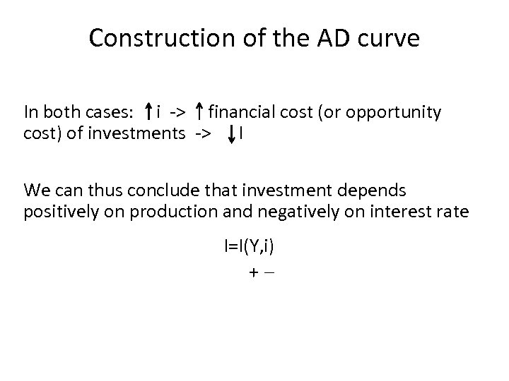Construction of the AD curve In both cases: i -> financial cost (or opportunity cost) of investments -> I We can thus conclude that investment depends positively on production and negatively on interest rate I=I(Y, i) +-

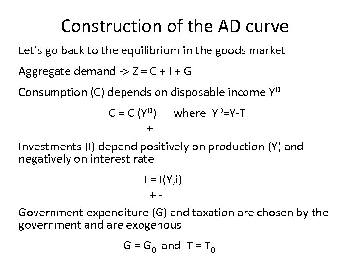Construction of the AD curve Let’s go back to the equilibrium in the goods market Aggregate demand -> Z = C + I + G Consumption (C) depends on disposable income YD C = C (YD) where YD=Y-T + Investments (I) depend positively on production (Y) and negatively on interest rate I = I(Y, i) +Government expenditure (G) and taxation are chosen by the government and are exogenous G = G 0 and T = T 0

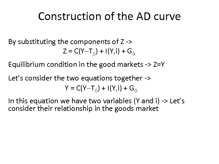Construction of the AD curve By substituting the components of Z -> Z = C(Y-T 0) + I(Y, i) + G 0 Equilibrium condition in the good markets -> Z=Y Let’s consider the two equations together -> Y = C(Y-T 0) + I(Y, i) + G 0 In this equation we have two variables (Y and i) -> Let’s consider their relationship in the goods market

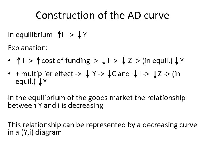Construction of the AD curve In equilibrium i -> Y Explanation: • i -> cost of funding -> • + multiplier effect -> equil. ) Y I -> Z -> (in equil. ) Y Y -> C and I -> Z -> (in In the equilibrium of the goods market the relationship between Y and i is decreasing This relationship can be represented by a decreasing curve in a (Y, i) diagram

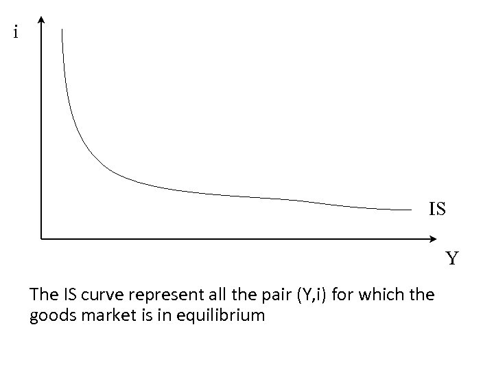i IS Y The IS curve represent all the pair (Y, i) for which the goods market is in equilibrium

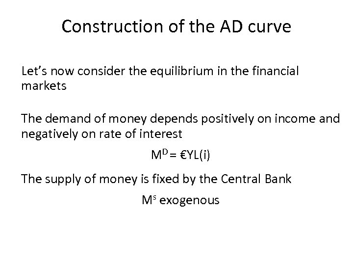Construction of the AD curve Let’s now consider the equilibrium in the financial markets The demand of money depends positively on income and negatively on rate of interest MD = €YL(i) The supply of money is fixed by the Central Bank Ms exogenous

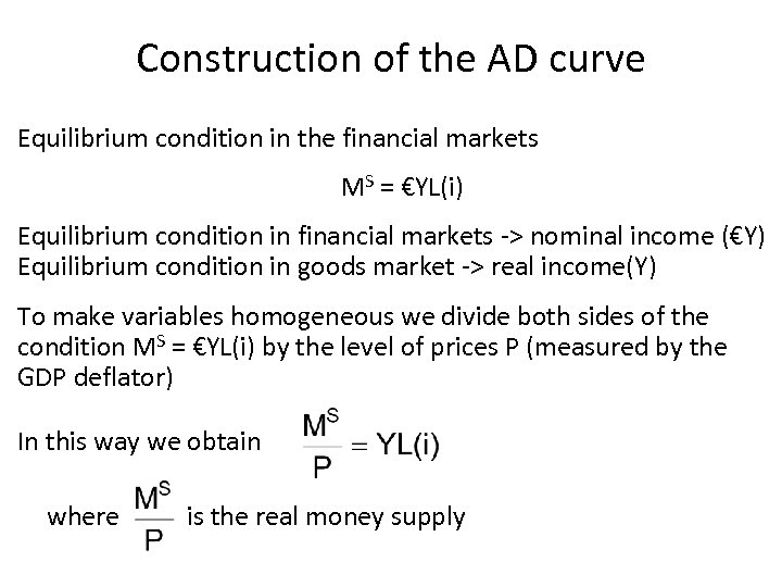Construction of the AD curve Equilibrium condition in the financial markets MS = €YL(i) Equilibrium condition in financial markets -> nominal income (€Y) Equilibrium condition in goods market -> real income(Y) To make variables homogeneous we divide both sides of the condition MS = €YL(i) by the level of prices P (measured by the GDP deflator) In this way we obtain where is the real money supply

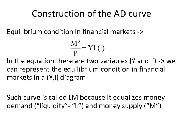Construction of the AD curve Equilibrium condition in financial markets -> In the equation there are two variables (Y and i) -> we can represent the equilibrium condition in financial markets in a (Y, i) diagram Such curve is called LM because it equalizes money demand (“liquidity”- “L”) and money supply (“M”)

Construction of the AD curve To construct the LM curve we consider the effects of an Y in financial markets In Lecture 12 we saw that Y -> i in equilibrium In equilibrium there is a positive relationship between Y and i -> The LM curve is upward sloping

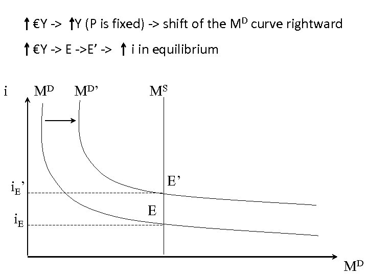€Y -> Y (P is fixed) -> shift of the MD curve rightward €Y -> E ->E’ -> i MD M D’ i in equilibrium MS E’ i. E E MD

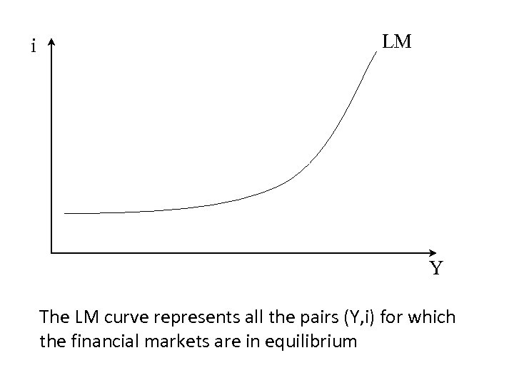i LM Y The LM curve represents all the pairs (Y, i) for which the financial markets are in equilibrium

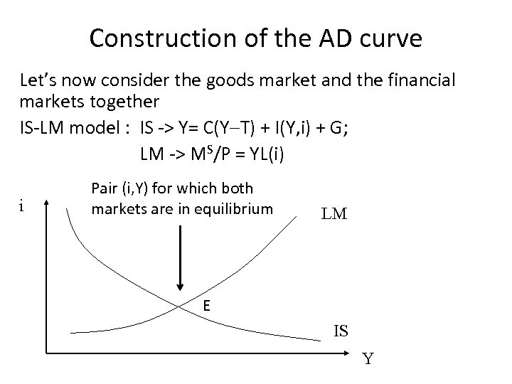Construction of the AD curve Let’s now consider the goods market and the financial markets together IS-LM model : IS -> Y= C(Y-T) + I(Y, i) + G; LM -> MS/P = YL(i) i Pair (i, Y) for which both markets are in equilibrium LM E IS Y

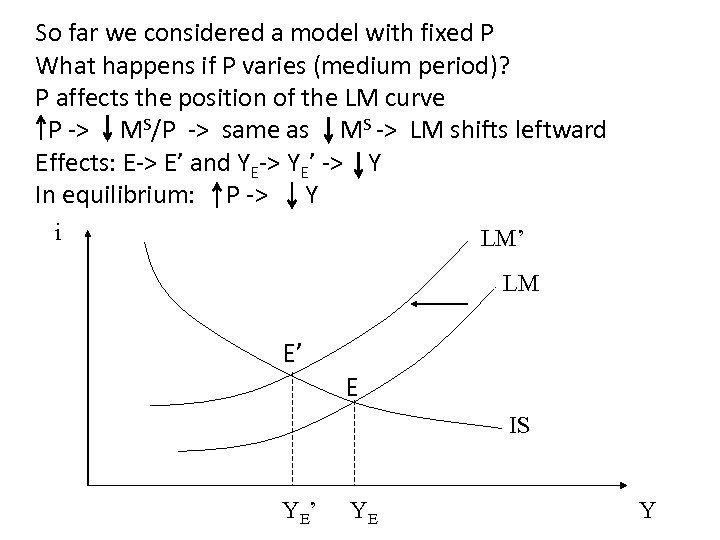So far we considered a model with fixed P What happens if P varies (medium period)? P affects the position of the LM curve P -> MS/P -> same as MS -> LM shifts leftward Effects: E-> E’ and YE-> YE’ -> Y In equilibrium: P -> Y i LM’ LM E’ E IS YE ’ YE Y

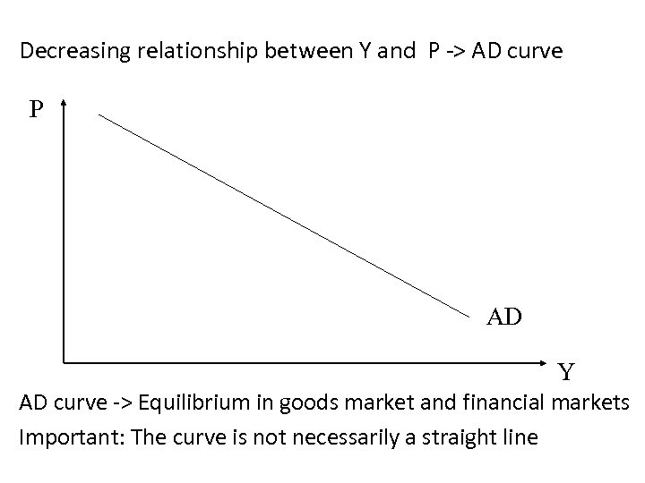Decreasing relationship between Y and P -> AD curve P AD Y AD curve -> Equilibrium in goods market and financial markets Important: The curve is not necessarily a straight line

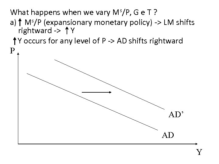What happens when we vary Ms/P, G e T ? a) Ms/P (expansionary monetary policy) -> LM shifts rightward -> Y Y occurs for any level of P -> AD shifts rightward P AD’ AD Y

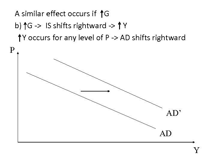A similar effect occurs if G b) G -> IS shifts rightward -> Y Y occurs for any level of P -> AD shifts rightward P AD’ AD Y

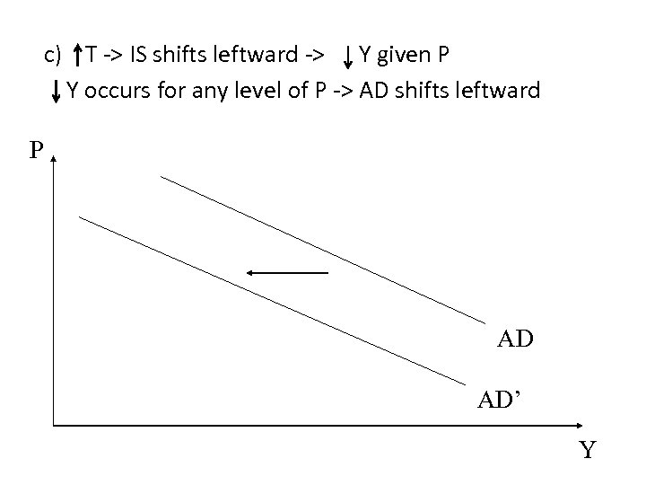c) T -> IS shifts leftward -> Y given P Y occurs for any level of P -> AD shifts leftward P AD AD’ Y

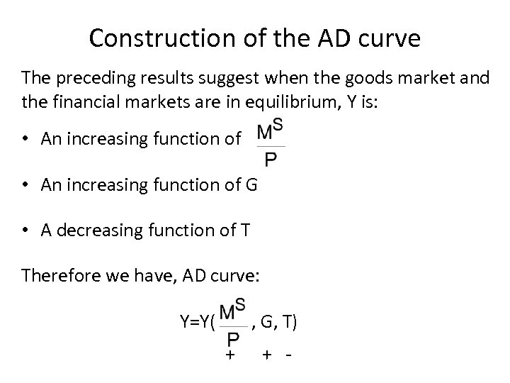Construction of the AD curve The preceding results suggest when the goods market and the financial markets are in equilibrium, Y is: • An increasing function of G • A decreasing function of T Therefore we have, AD curve: Y=Y( , G, T) + + -

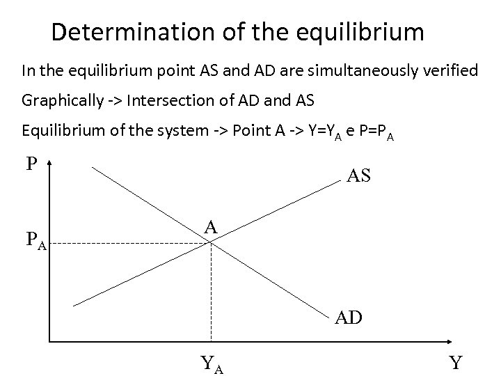Determination of the equilibrium In the equilibrium point AS and AD are simultaneously verified Graphically -> Intersection of AD and AS Equilibrium of the system -> Point A -> Y=YA e P=PA P PA AS A AD YA Y

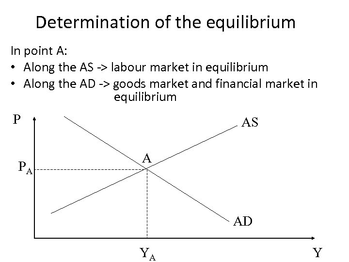Determination of the equilibrium In point A: • Along the AS -> labour market in equilibrium • Along the AD -> goods market and financial market in equilibrium P PA AS A AD YA Y

Determination of the equilibrium Point A can represent the equilibrium both in the short and in the medium period, depending on the assumption on PE The position of A, indeed, depends on the position of the AS curve and thus on PE In particular : • Medium period, PE=P -> u=un -> Y=Yn In the medium period equilibrium Y is always equal to Yn • Short period, PE can be ≠ P -> Y ≠ Yn Three cases: PE=P -> Y=Yn ; PE>P -> Y Y>Yn

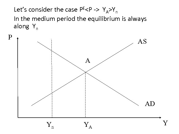Let’s consider the case PE

YA>Yn In the medium period the equilibrium is always along Yn P AS A AD Yn YA Y

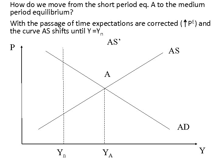How do we move from the short period eq. A to the medium period equilibrium? With the passage of time expectations are corrected ( PE) and the curve AS shifts until Y =Yn AS’ P AS A AD Yn YA Y

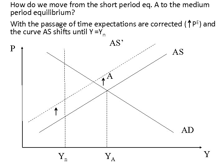How do we move from the short period eq. A to the medium period equilibrium? With the passage of time expectations are corrected ( PE) and the curve AS shifts until Y =Yn AS’ P AS A AD Yn YA Y

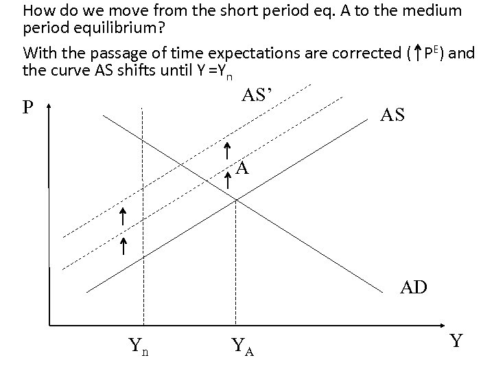How do we move from the short period eq. A to the medium period equilibrium? With the passage of time expectations are corrected ( PE) and the curve AS shifts until Y =Yn AS’ P AS A AD Yn YA Y

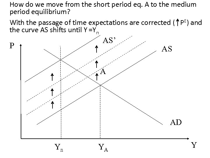How do we move from the short period eq. A to the medium period equilibrium? With the passage of time expectations are corrected ( PE) and the curve AS shifts until Y =Yn AS’ P AS A AD Yn YA Y

Conclusion Combining goods market, financial market and labour market we studied the determination of equilibrium in the medium period. The main difference with the short period is that now price can vary (+ investment are endogenous). The AD-AS model is the main macroeconomic model that is used to investigate the effect of policy interventions.

Next AD-AS exercises and applications