c0103b08db292db005096805fb120029.ppt
- Количество слайдов: 54
Texture Analysis and Synthesis – Seminar Semester B, 2006 -2007 Presented by Eyal Gilstron
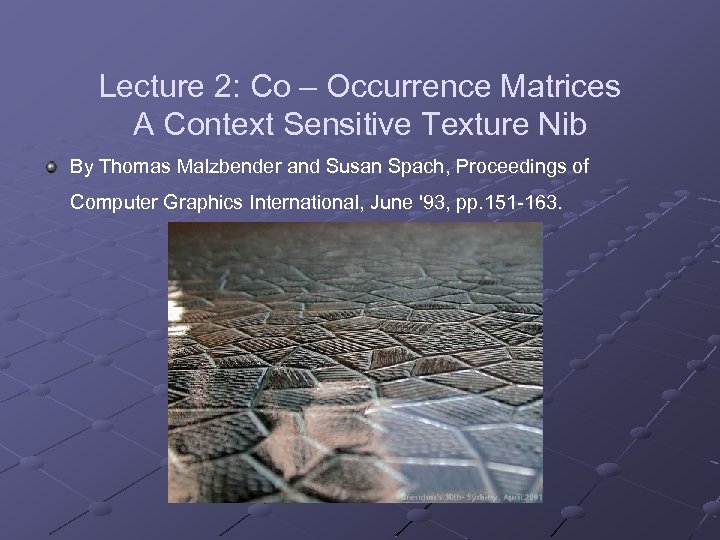
Lecture 2: Co – Occurrence Matrices A Context Sensitive Texture Nib By Thomas Malzbender and Susan Spach, Proceedings of Computer Graphics International, June '93, pp. 151 -163.
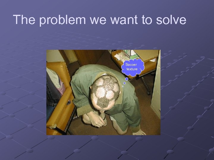
The problem we want to solve Soccer texture
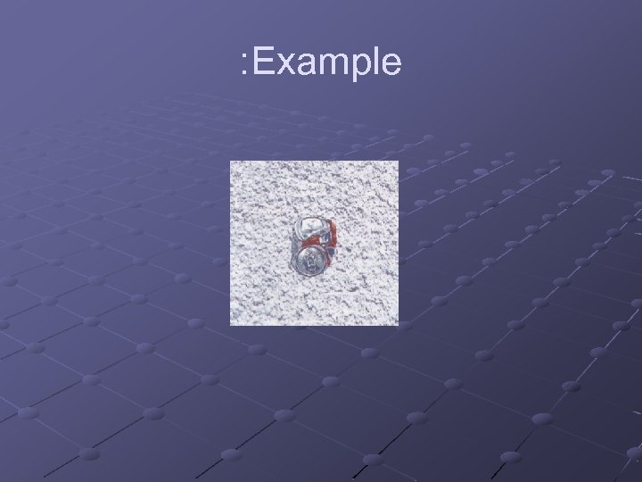
Problem: We have an Image which has a interesting texture and we want to remove other object in interactive matter (i. e. manual eraser behavior).
: Example
History and old techniques
Lets go back in time and try to remember. .
Histogram Image processing – Lesson 2 – Hagit Hal-Or
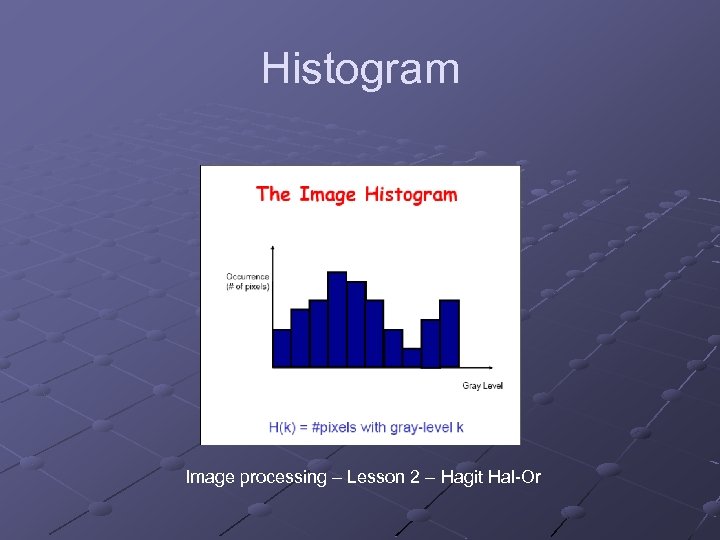
'Houston, We Have a Problem!' Two equal histograms may represent two very dissimilar images. Histograms is a point operation so we just know how many pixs we have in each gray scale color, It’s not a geometric operation. Maybe we need another tool which can represent also spatial data (point & geometric). Remember this problem!

GLCM and GCM Before we will get to GCM, we will talk about a simpler algorithm, GLCM.
GLCM The idea behind GLCM is to describe the texture as a matrix of “pair gray level probabilities”. This allows us to know which gray-level pairs, a texture is more dominant are more dominant and which are less, and may allow us (hopefully) to stochasitcally grow the texture by randomly deciding pixel colors according to those probabilities.
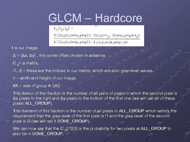
GLCM – Hardcore I is our image. Δ = {Δx, Δy} , this some offset chosen in advance. C Δ= a matrix. i 1, i 2 – these are the indices to our matrix, which are also grey-level values. n – width and height of our image. #A – size of group A (|A|) The divisor of this fraction is the number of all pairs of pixels in which the second pixel is Δx pixels to the right and Δy pixels to the bottom of the first one (we will call of these pixels ALL_GROUP). The dividend of this fraction is the number of all pixels in ALL_GROUP which satisfy the requirement that the gray-level of the first pixel is i 1 and the gray-level of the second pixel is i 2 (we will call it SOME_GROUP). We can now say that the C Δ[i 1][i 2] is the probability for two pixels at ALL_GROUP to also be in SOME_GROUP.
GLCM – Why is it useful? The matrix seen here can be used to find out probabilities of some texture features to appear, which allows us to get an image of how the texture “behaves”. Example: probability of two pixels having a difference in gray-level d: take the sum of a diagonal line in the matrix which starts from GLCM[0][d] to find out the probability of two pixels having difference d between them.
GCM – A generalization
GCM – A generalization The idea represented in GLCM is a good idea when we want to work with probabilities of gray levels of pixels. Sometimes we are interested in something else, sometimes we don’t even consider an image as a collection of pixels with gray -levels, but as “something else”. GCM allows us to formally define “something else”.
GCM - Components p – a collection of attributes representing an “image element”. Examples: ppixel = {position, gray-level} (“simple” pixels) pedge={position, intensity, direction} (output of edge detection) S – a function which gets two p-elements and returns either true or false. Examples: (f 1, f 2 are “objects” of “type” p) spixel(f 1, f 2) = true f 2. position – f 1. position = (Δx, Δy) f 2. position – f 1. position = sedge(f 1, f 2) = true abs(f 2. position – f 1. position) ≤ 20) A – some attribute of p which “interests” us.
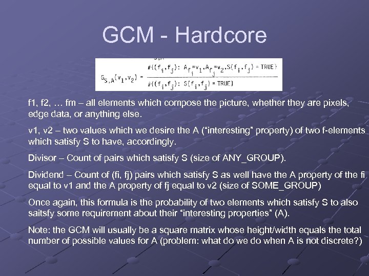
GCM - Hardcore f 1, f 2, … fm – all elements which compose the picture, whether they are pixels, edge data, or anything else. v 1, v 2 – two values which we desire the A (“interesting” property) of two f-elements which satisfy S to have, accordingly. Divisor – Count of pairs which satisfy S (size of ANY_GROUP). Dividend – Count of (fi, fj) pairs which satisfy S as well have the A property of the fi equal to v 1 and the A property of fj equal to v 2 (size of SOME_GROUP) Once again, this formula is the probability of two elements which satisfy S to also saitsfy some requirement about their “interesting properties” (A). Note: the GCM will usually be a square matrix whose height/width equals the total number of possible values for A (problem: what do we do when A is not discrete? )
GCM – Generalization of GLCM It is easy to see that GCM is a generalization of GLCM, in fact, this has already been showed to you before, let’s look at the following definitions: ppixel = {position, gray-level} (“simple” pixels) spixel(f 1, f 2) = true f 2. position – f 1. position = (Δx, Δy)=Δ Apixel=gray-level If you go back to the GCM formula you can see that if we define (p, s, a), we get GLCM.

Example on board. .
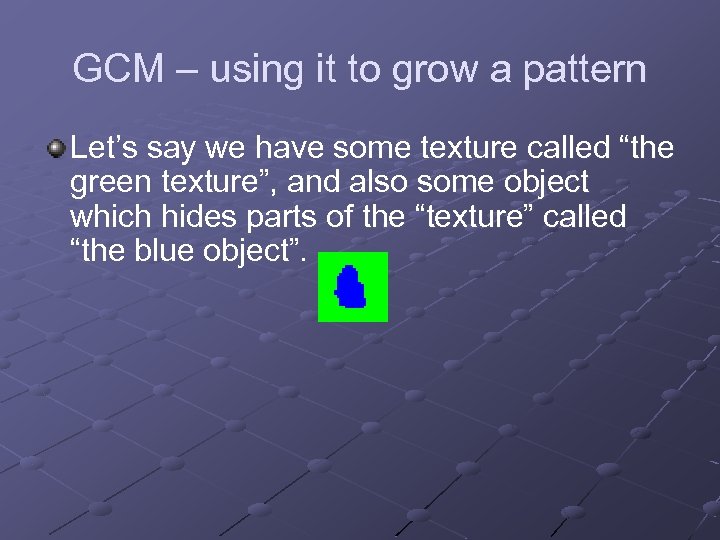
GCM – using it to grow a pattern Let’s say we have some texture called “the green texture”, and also some object which hides parts of the “texture” called “the blue object”.
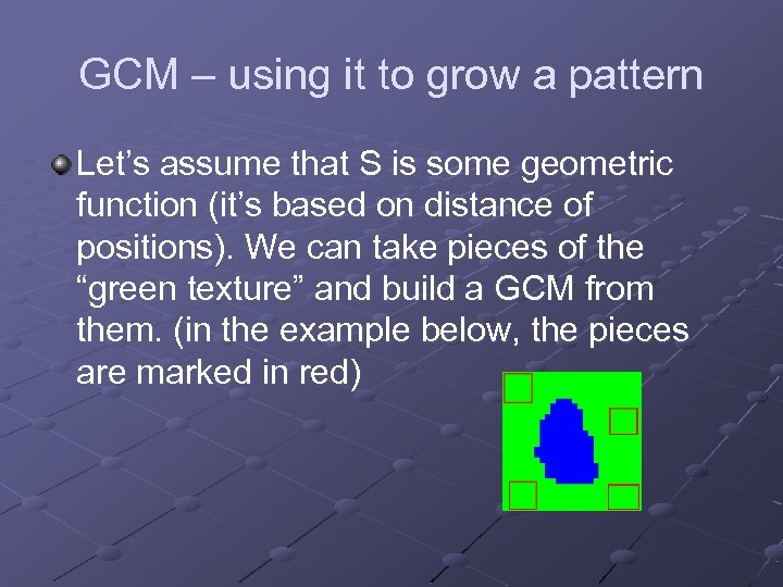
GCM – using it to grow a pattern Let’s assume that S is some geometric function (it’s based on distance of positions). We can take pieces of the “green texture” and build a GCM from them. (in the example below, the pieces are marked in red)
GCM – using it to grow a pattern We can then stochastically replace points of “the blue object” with points generated based on the probabilities in the GCM. Let’s say we have two points which satisfy S, one is in “the green texture” and one is in “the blue object”. We can replace the A property of S (let’s assume A is ‘color’) with something which would fit “the green texture”.
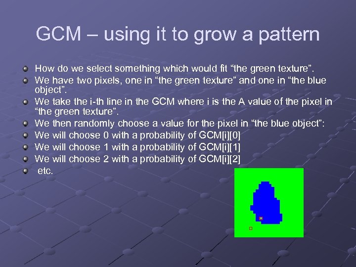
GCM – using it to grow a pattern How do we select something which would fit “the green texture”. We have two pixels, one in “the green texture” and one in “the blue object”. We take the i-th line in the GCM where i is the A value of the pixel in “the green texture”. We then randomly choose a value for the pixel in “the blue object”: We will choose 0 with a probability of GCM[i][0] We will choose 1 with a probability of GCM[i][1] We will choose 2 with a probability of GCM[i][2] etc.
A Fast Method to Determine Co-Occurrence Texture Features Using A Linked List Implementation One of the basic rules in practical computer sciences is: “if it can’t be done fast, it can’t be done at all”. GLCM matrices have two characteristics: 1) They are big. 2) They are sparse. Since they are big, in most cases we do not have to calculate the entire matrix, but can instead “lazy-evaluate” only the parts we need. It would still be smart to store the results of those “lazy evaulations”. However, eventually we may still have to store a large amount of data in the memory. Luckily, the matrices are also usually sparse, which means that instead of storing the matrix, we can only store the coordinates and values of places in the matrix which are not zero. This can be possibly done via a linked list (in my opinion, for better performance it would be wise to use a hash map).
Color Co–Occurrence Matrix - CCM
Malzbender and Spach technique “Our technique is based on mimicking a second order statistics of samples of scanned textures, typically taken from photographs of real textures occurring in nature. We use Color Co. Occurrence Matrices to capture and optimized these second order statistics. This technique is shown to provide interactive response and good performance over a broad range of stationary textures, from periodic to stochastic. ”
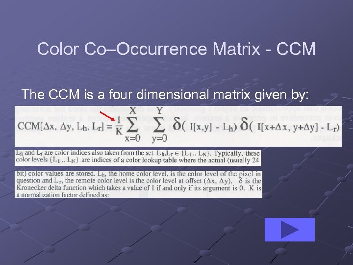
Color Co–Occurrence Matrix - CCM The CCM is a four dimensional matrix given by:
Color Co–Occurrence Matrix - CCM
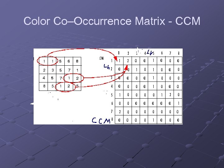
Color Co–Occurrence Matrix - CCM To illustrate, the following figure shows how graycomatrix calculates the first three values in a CCM. In the output CCM , element (1, 1) contains the value 1 because there is only one instance in the input image where two horizontally adjacent pixels have the values 1 and 1, respectively. glcm(1, 2) contains the value 2 because there are two instances where two horizontally adjacent pixels have the values 1 and 2. Element (1, 3) in the CCM has the value 0 because there are no instances of two horizontally adjacent pixels with the values 1 and 3. graycomatrix continues processing the input image, scanning the image for other pixel pairs (i, j) and recording the sums in the corresponding elements of the CCM.
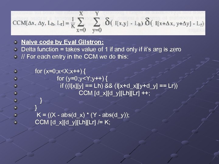
Naive code by Eyal Gilstron: Delta function = takes value of 1 if and only if it’s arg is zero // For each entry in the CCM we do this: for (x=0; x<X; x++) { for (y=0; y<Y; y++) { if ((I[x][y] == Lh) && (I[x+d_x][y+d_y] == Lr)) CCM [d_x][d_y][Lh][Lr] ++; } } K = ((X - abs(d_x) * (Y - abs(d_y)); CCM [d_x][d_y][Lh][Lr] /= K;
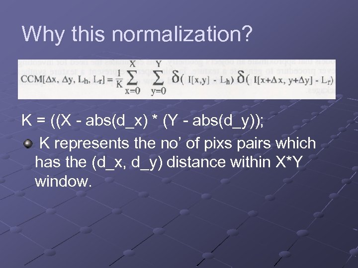
Why this normalization? K = ((X - abs(d_x) * (Y - abs(d_y)); K represents the no’ of pixs pairs which has the (d_x, d_y) distance within X*Y window.
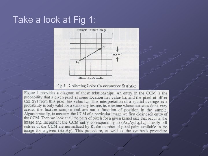
Take a look at Fig 1:
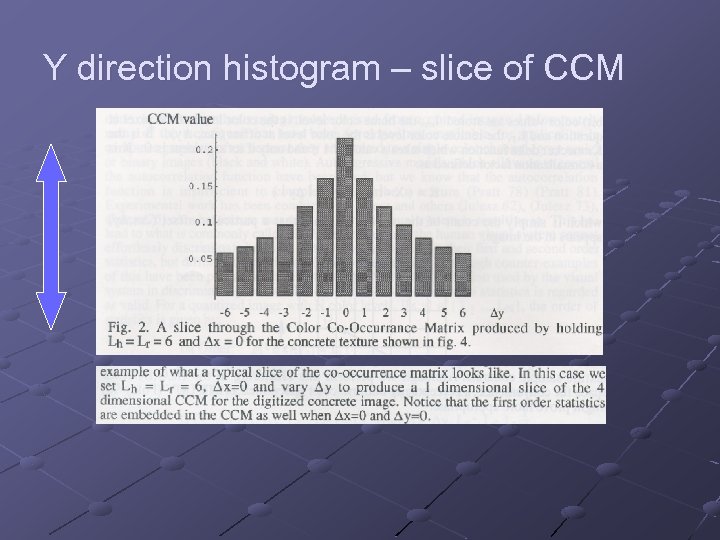
Y direction histogram – slice of CCM
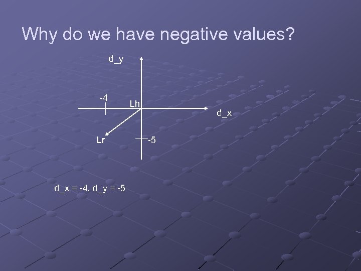
Why do we have negative values? d_y -4 Lr d_x = -4, d_y = -5 Lh d_x -5
Color Quantization CCM size can be extremely large when we use colors instead of grayscale: (2 * d_XMAX +1) * (2 * d_YMAX +1) * N N = number of chosen colors (“This color {L 1 . . LN} are indices of color lookup table of 24 bit colors”) If we use all 24 bit possible colors CCM it’s unpractical.
Color Quantization continue Actually we can have small set of colors and still retain excellent texture image quality. There are many methods for picking subset of colors. We choose the K-means (avg) clustering (Lim 90) (see more " "מערכות דימות וצבע course by Hagit Hal-Or)
Texture Nib Question: What is a Texture Nib? Answer: Texture Nib is an application. Question: So how does it work? Answer: patience my friends.
Texture Nib Application

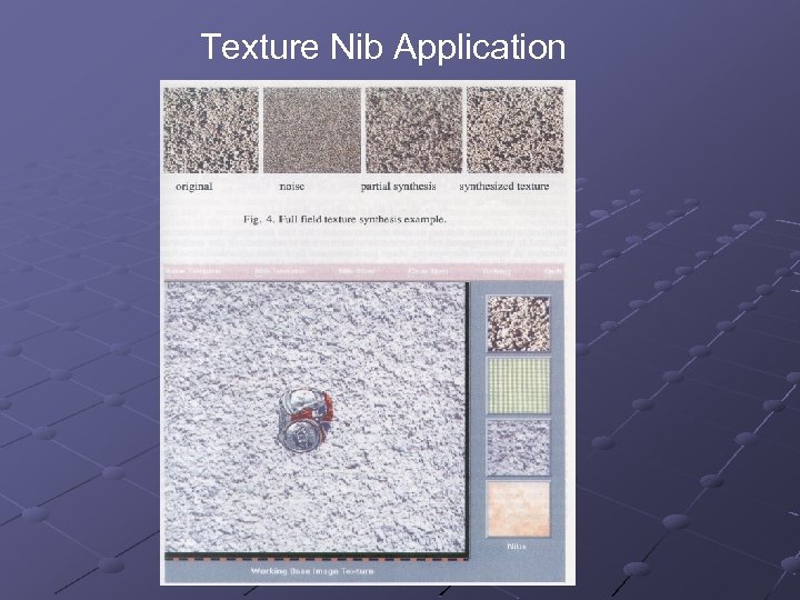
User point of view: We have a texture image that contains a crushed soda can, we want to remove the soda can and refill with the texture. So we pick a window from the image with the texture that will be the reference. We define a ‘nib’ cursor and we start scroll the soda can until it is removed.
How the nib texture algorithm works? For using the nib texture the user defines a nib size (window) and CCM size. First, the program fills the nib window with noise then it updates the CCM in the relevant entries and after it calculates the Euclidian distance between the destination (base texture), and the current nib texture, to determine how close we are. Iteratively the program changes the colors in the nib until we minimize the error.
Define matrices CCMd = Our destination (see texture nib) CCMw = Working CCMt = Our try CCM – result of color changing according to CCMw
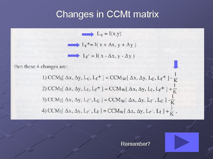
Changes in CCMt matrix Why? Remember?
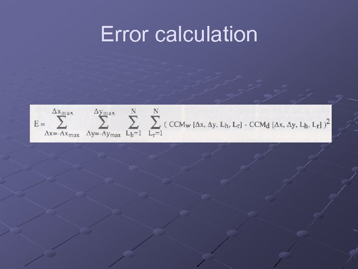
Error calculation
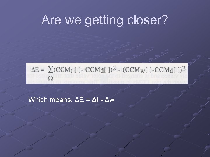
Are we getting closer? Which means: ΔE = Δt - Δw
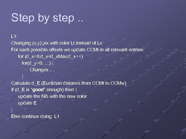
Step by step. . L 1: Changing (x, y) pix with color Lt instead of Lc For each possible offsets we update CCMt in all relevant entries: for (d_x=0; d_x<d_x. Max; d_x++) for(d_y=0; …) { Changes … } Calculate d_E (Euclidian distance from CCMt to CCMw) If (d_E is “good” enough) then { update the Nib with the new color update E } Else continue doing L 1
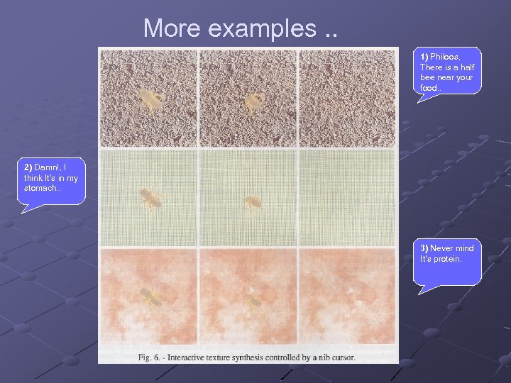
More examples. . 1) Philoos, There is a half bee near your food. . 2) Damn!, I think It’s in my stomach. . 3) Never mind It’s protein.
Small world. .
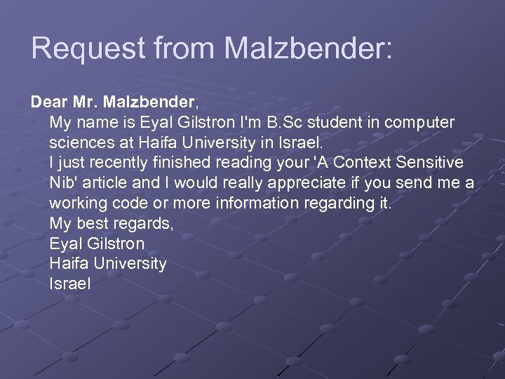
Request from Malzbender: Dear Mr. Malzbender, My name is Eyal Gilstron I'm B. Sc student in computer sciences at Haifa University in Israel. I just recently finished reading your 'A Context Sensitive Nib' article and I would really appreciate if you send me a working code or more information regarding it. My best regards, Eyal Gilstron Haifa University Israel

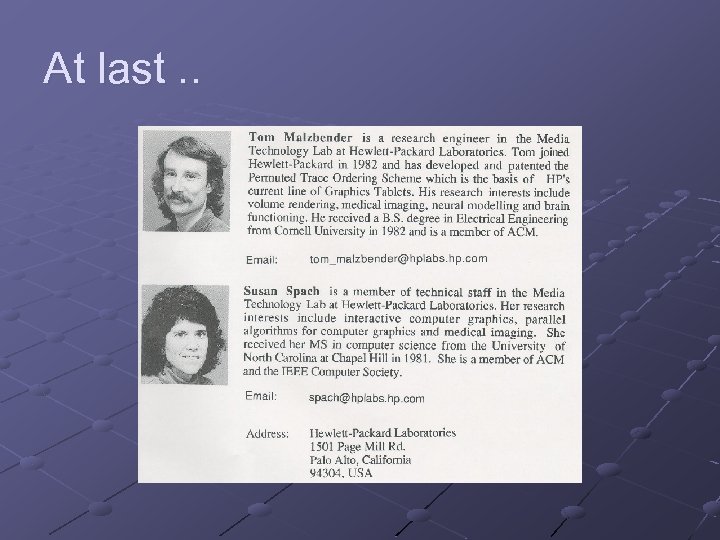
What a small world. . Eyal, The texture nib work is very old and the code I have I wrote on a HP UX system. I've attached what I have, but don't know if it will compile as is. I do think there is a possibility of a larger publication with this sort of approach. No interactive texture synthesis has been presented at Siggraph yet. Also, there is a person in Haifa who I have worked with who has interest in this work, his name is Jacov Hel-Or. I would recommend contacting him, bright guy. regards, Tom
At last. .

The End. Bye. .
c0103b08db292db005096805fb120029.ppt