845283204475b3136a8c01b2eb17c3ed.ppt
- Количество слайдов: 44
 Technion Israel Institute of Technology Computer Science Department Efficient Keyword Search Over Virtual XML Views Authors: Feng Shao, Lin Guo, Chavadar Botev, Anand Bhaskar, Muthiah Chettiar, Fan Yang Tal Herscovitz
 Outline Motivation and Problem Definition Existing Data and Data Structures Algorithm Experiments
 Personalized Portal my. yahoo. com
 The Problem… Traditional information retrieval systems rely heavily on the assumption that the set of documents being searched is materialized.
 Materialized XML Views? We might not have the resources to materialize all the data If the view is materialized, its contents might be out of date Data sources might not wish to provide the entire dataset The problem
 Materialized XML Views? Tradeoff How do we efficiently evaluate keyword search queries over virtual XML views? How do we return only the top ranked results to the user?
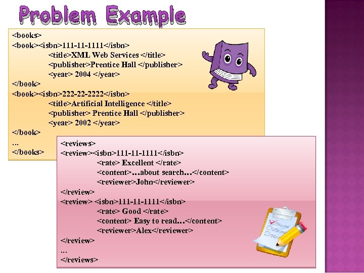 Problem Example
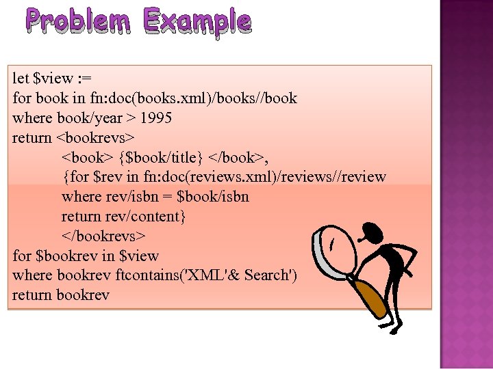 Problem Example let $view : = for book in fn: doc(books. xml)/books//book where book/year > 1995 return
 Problem Example
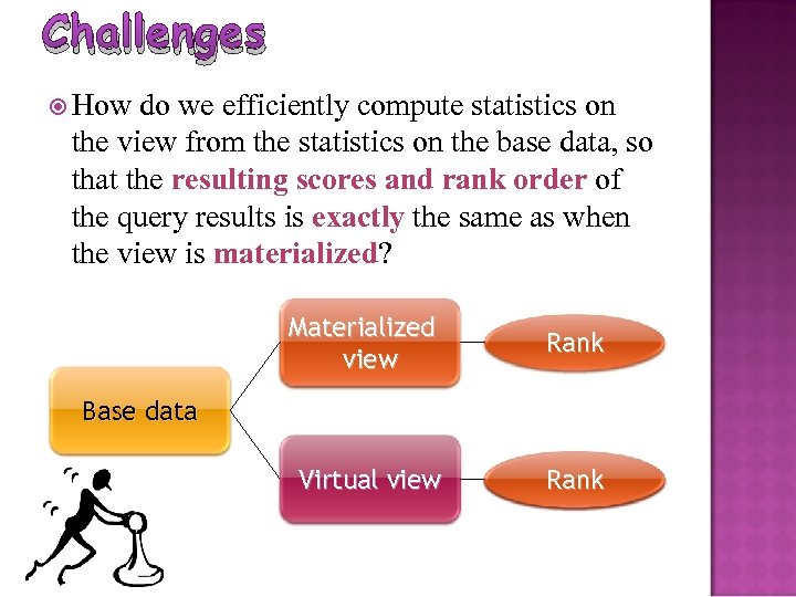 Challenges How do we efficiently compute statistics on the view from the statistics on the base data, so that the resulting scores and rank order of the query results is exactly the same as when the view is materialized? Materialized view Rank Virtual view Rank Base data
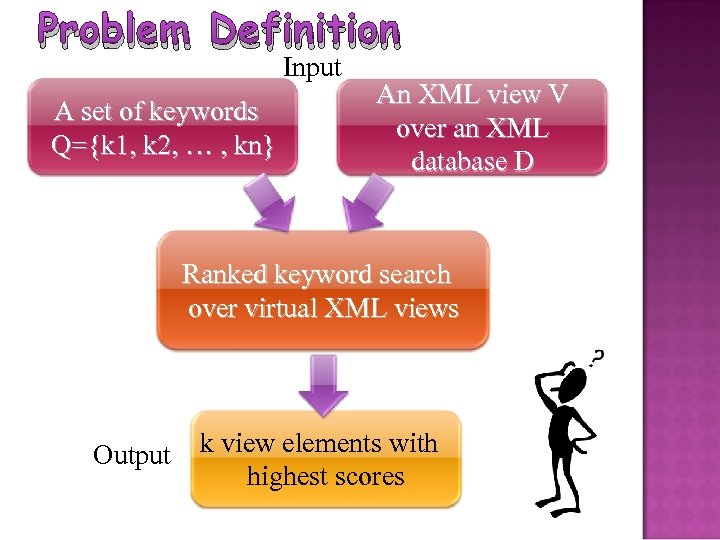 Problem Definition Input A set of keywords Q={k 1, k 2, … , kn} An XML view V over an XML database D Ranked keyword search over virtual XML views Output k view elements with highest scores
 Outline Motivation and Problem Definition Existing Data and Data Structures Algorithm Experiments
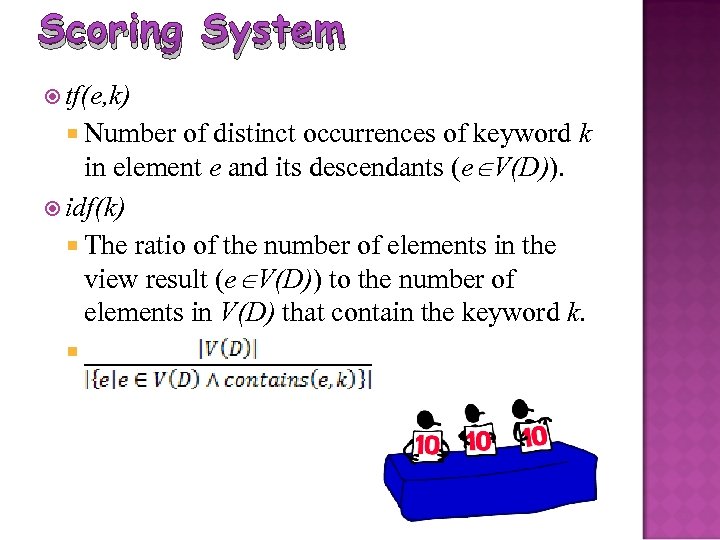 Scoring System tf(e, k) Number of distinct occurrences of keyword k in element e and its descendants (e V(D)). idf(k) The ratio of the number of elements in the view result (e V(D)) to the number of elements in V(D) that contain the keyword k.
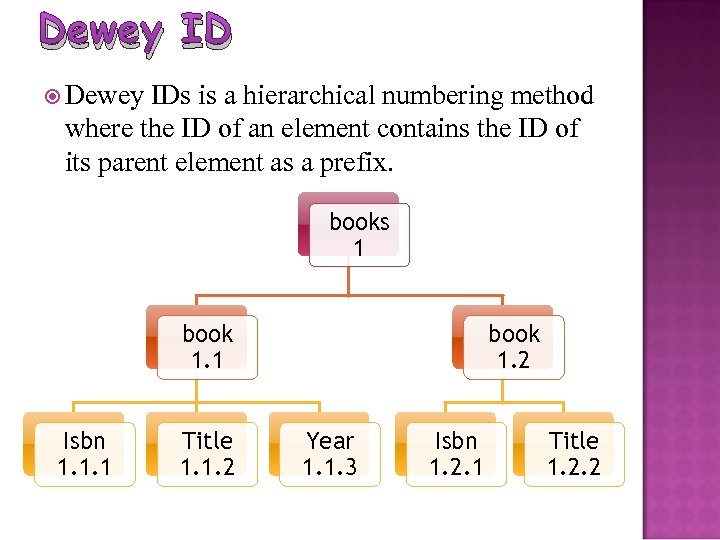 Dewey ID Dewey IDs is a hierarchical numbering method where the ID of an element contains the ID of its parent element as a prefix. books 1 book 1. 1 Isbn 1. 1. 1 Title 1. 1. 2 book 1. 2 Year 1. 1. 3 Isbn 1. 2. 1 Title 1. 2. 2
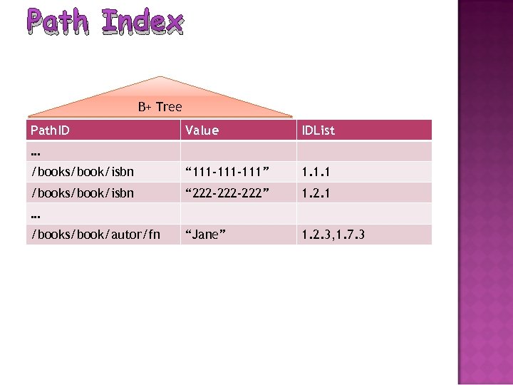 Path Index B+ Tree Path. ID Value IDList /books/book/isbn “ 111 -111” 1. 1. 1 /books/book/isbn “ 222 -222” 1. 2. 1 “Jane” 1. 2. 3, 1. 7. 3 … … /books/book/autor/fn
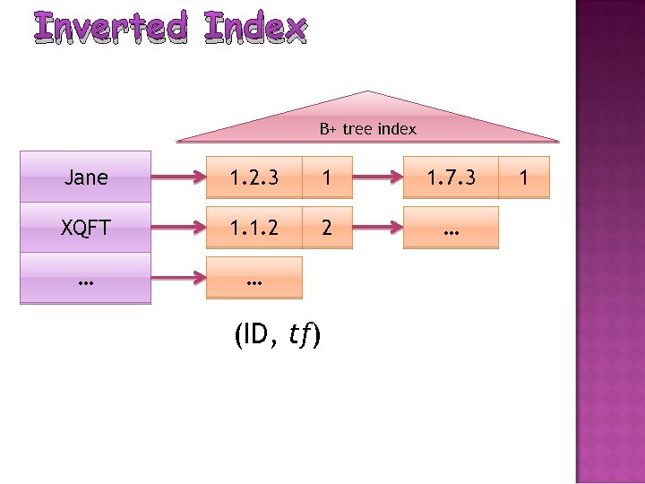 Inverted Index B+ tree index Jane 1. 2. 3 1 1. 7. 3 XQFT 1. 1. 2 2 … … … (ID, tf) 1
 Outline Motivation and Problem Definition Existing Data and Data Structures Algorithm Experiments
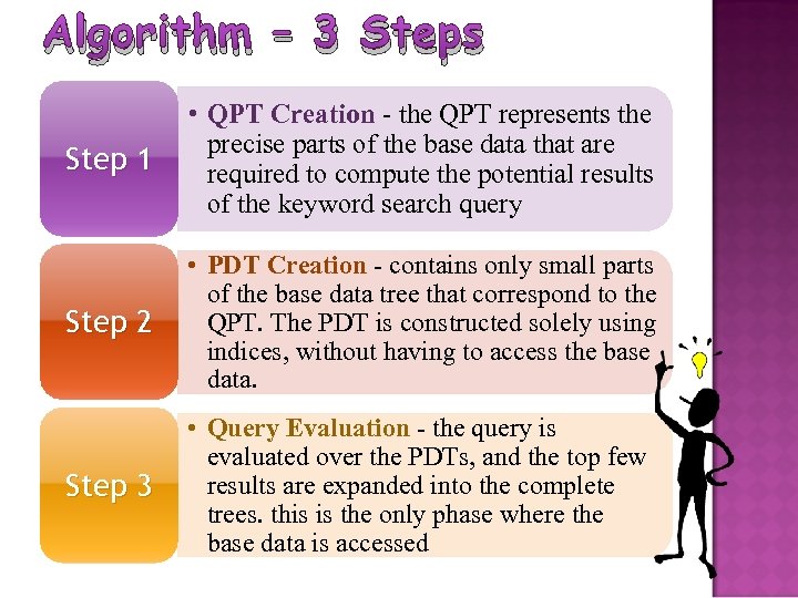 Algorithm – 3 Steps Step 1 • QPT Creation - the QPT represents the precise parts of the base data that are required to compute the potential results of the keyword search query Step 2 • PDT Creation - contains only small parts of the base data tree that correspond to the QPT. The PDT is constructed solely using indices, without having to access the base data. Step 3 • Query Evaluation - the query is evaluated over the PDTs, and the top few results are expanded into the complete trees. this is the only phase where the base data is accessed
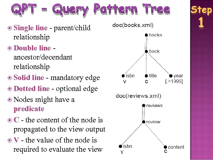 QPT – Query Pattern Tree Single line - parent/child relationship Double line ancestor/decendant relationship Solid line - mandatory edge Dotted line - optional edge Nodes might have a predicate C - the content of the node is propagated to the view output V - the value of the node is required to evaluate the view Step 1
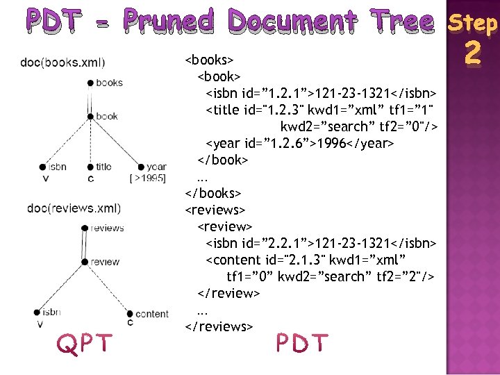 PDT - Pruned Document Tree
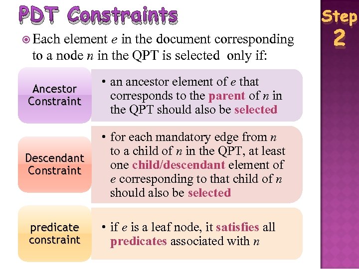 PDT Constraints Each element e in the document corresponding to a node n in the QPT is selected only if: Ancestor Constraint • an ancestor element of e that corresponds to the parent of n in the QPT should also be selected Descendant Constraint • for each mandatory edge from n to a child of n in the QPT, at least one child/descendant element of e corresponding to that child of n should also be selected predicate constraint • if e is a leaf node, it satisfies all predicates associated with n Step 2
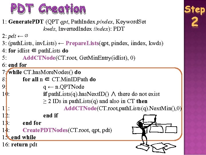
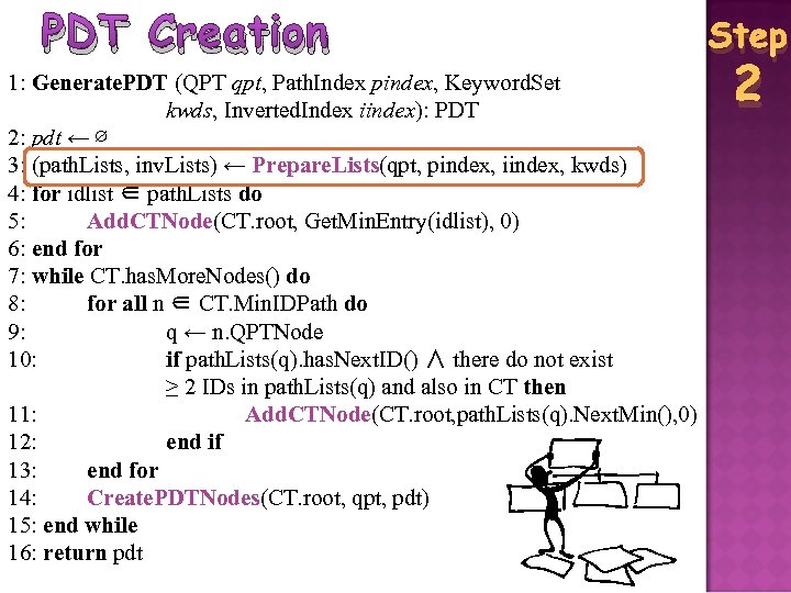 PDT Creation 1: Generate. PDT (QPT qpt, Path. Index pindex, Keyword. Set kwds, Inverted. Index iindex): PDT 2: pdt ← ∅ 3: (path. Lists, inv. Lists) ← Prepare. Lists(qpt, pindex, iindex, kwds) 4: for idlist ∈ path. Lists do 5: Add. CTNode(CT. root, Get. Min. Entry(idlist), 0) 6: end for 7: while CT. has. More. Nodes() do 8: for all n ∈ CT. Min. IDPath do 9: q ← n. QPTNode 10: if path. Lists(q). has. Next. ID() ∧ there do not exist ≥ 2 IDs in path. Lists(q) and also in CT then 11: Add. CTNode(CT. root, path. Lists(q). Next. Min(), 0) 12: end if 13: end for 14: Create. PDTNodes(CT. root, qpt, pdt) 15: end while 16: return pdt Step 2
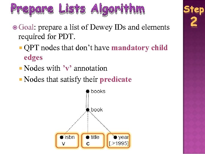 Prepare Lists Algorithm Goal: prepare a list of Dewey IDs and elements required for PDT. QPT nodes that don’t have mandatory child edges Nodes with ’v’ annotation Nodes that satisfy their predicate Step 2
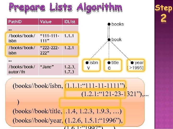 Prepare Lists Algorithm Path. ID Value IDList /books/book/ isbn “ 111 -111111” 1. 1. 1 /books/book/ isbn “ 222 -222222” 1. 2. 1 “Jane” 1. 2. 3, 1. 7. 3 … … /books/book/ autor/fn (books//book/isbn, (1. 1. 1: “ 111 -11 -1111”), (1. 2. 1: “ 121 -23 -1321”), . . . ) (books//book/title, 1. 1. 4, 1. 2. 3, 1. 9. 3, …) (books//book/year, (1. 2. 6, 1. 5. 1: “ 1996”), Step 2
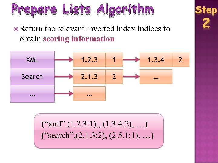 Prepare Lists Algorithm Step 2 Return the relevant inverted index indices to obtain scoring information XML 1. 2. 3 1 1. 3. 4 Search 2. 1. 3 2 … … … (“xml”, (1. 2. 3: 1), , (1. 3. 4: 2), …) (“search”, (2. 1. 3: 2), (2. 5. 1: 1), …) 2
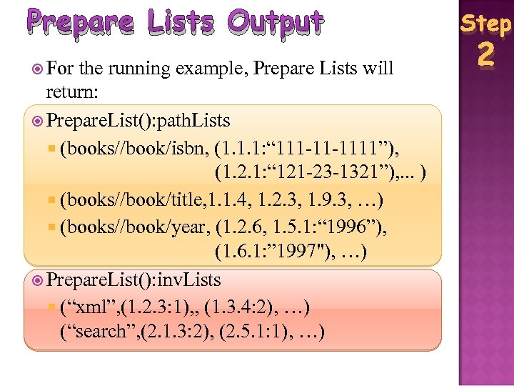 Prepare Lists Output For the running example, Prepare Lists will return: Prepare. List(): path. Lists (books//book/isbn, (1. 1. 1: “ 111 -11 -1111”), (1. 2. 1: “ 121 -23 -1321”), . . . ) (books//book/title, 1. 1. 4, 1. 2. 3, 1. 9. 3, …) (books//book/year, (1. 2. 6, 1. 5. 1: “ 1996”), (1. 6. 1: ” 1997"), …) Prepare. List(): inv. Lists (“xml”, (1. 2. 3: 1), , (1. 3. 4: 2), …) (“search”, (2. 1. 3: 2), (2. 5. 1: 1), …) Step 2
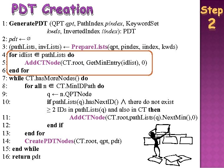 PDT Creation 1: Generate. PDT (QPT qpt, Path. Index pindex, Keyword. Set kwds, Inverted. Index iindex): PDT 2: pdt ← ∅ 3: (path. Lists, inv. Lists) ← Prepare. Lists(qpt, pindex, iindex, kwds) 4: for idlist ∈ path. Lists do 5: Add. CTNode(CT. root, Get. Min. Entry(idlist), 0) 6: end for 7: while CT. has. More. Nodes() do 8: for all n ∈ CT. Min. IDPath do 9: q ← n. QPTNode 10: if path. Lists(q). has. Next. ID() ∧ there do not exist ≥ 2 IDs in path. Lists(q) and also in CT then 11: Add. CTNode(CT. root, path. Lists(q). Next. Min(), 0) 12: end if 13: end for 14: Create. PDTNodes(CT. root, qpt, pdt) 15: end while 16: return pdt Step 2
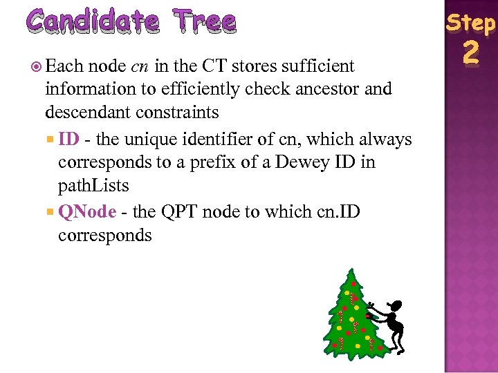 Candidate Tree Each node cn in the CT stores sufficient information to efficiently check ancestor and descendant constraints ID - the unique identifier of cn, which always corresponds to a prefix of a Dewey ID in path. Lists QNode - the QPT node to which cn. ID corresponds Step 2
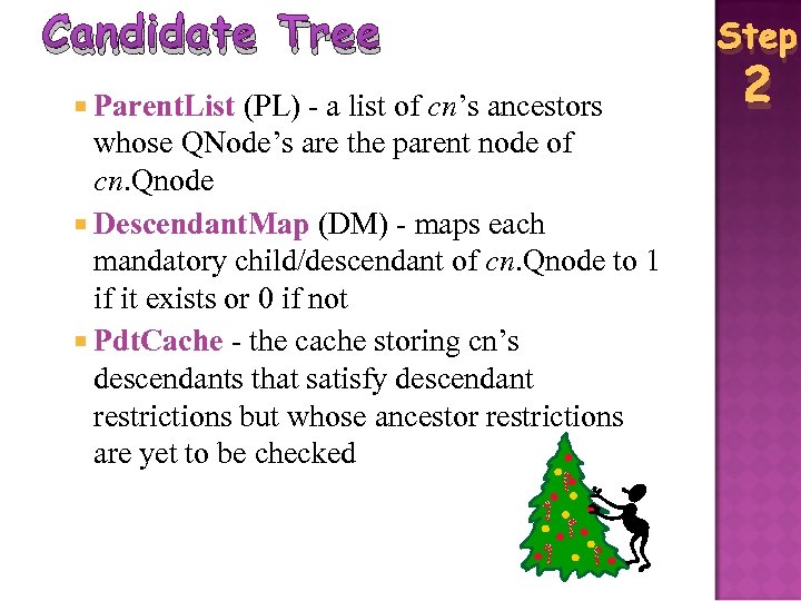 Candidate Tree Parent. List (PL) - a list of cn’s ancestors whose QNode’s are the parent node of cn. Qnode Descendant. Map (DM) - maps each mandatory child/descendant of cn. Qnode to 1 if it exists or 0 if not Pdt. Cache - the cache storing cn’s descendants that satisfy descendant restrictions but whose ancestor restrictions are yet to be checked Step 2
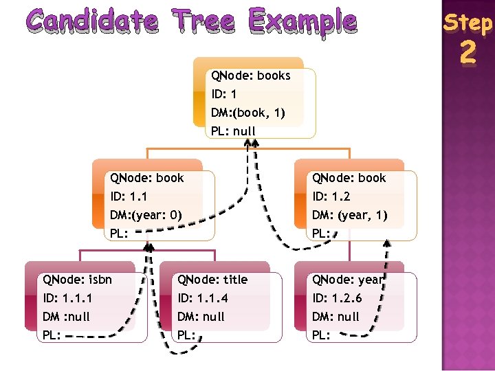 Candidate Tree Example QNode: books ID: 1 DM: (book, 1) PL: null QNode: book ID: 1. 1 DM: (year: 0) PL: ID: 1. 2 DM: (year, 1) PL: QNode: isbn QNode: title QNode: year ID: 1. 1. 1 DM : null PL: ID: 1. 1. 4 DM: null PL: ID: 1. 2. 6 DM: null PL: Step 2
 Add. CTNode Algorithm A prefix is added to the CT if it has a corresponding QPT node and is not already in the CT If a prefix is associated with a ’c’ annotation, the tf values are retrieved from the inverted lists Step 2
 PDT Creation 1: Generate. PDT (QPT qpt, Path. Index pindex, Keyword. Set kwds, Inverted. Index iindex): PDT 2: pdt ← ∅ 3: (path. Lists, inv. Lists) ← Prepare. Lists(qpt, pindex, iindex, kwds) 4: for idlist ∈ path. Lists do 5: Add. CTNode(CT. root, Get. Min. Entry(idlist), 0) 6: end for 7: while CT. has. More. Nodes() do 8: for all n ∈ CT. Min. IDPath do 9: q ← n. QPTNode 10: if path. Lists(q). has. Next. ID() ∧ there do not exist ≥ 2 IDs in path. Lists(q) and also in CT then 11: Add. CTNode(CT. root, path. Lists(q). Next. Min(), 0) 12: end if 13: end for 14: Create. PDTNodes(CT. root, qpt, pdt) 15: end while 16: return pdt Step 2
 The Main Loop Adds new Dewey IDs to the CT Creates PDT nodes using CT nodes Every iteration ensures that the Dewey IDs that are processed and known to be PDT nodes, are either in the CT or in the result PDT The result PDT only contains IDs that satisfy the PDT definition Step 2
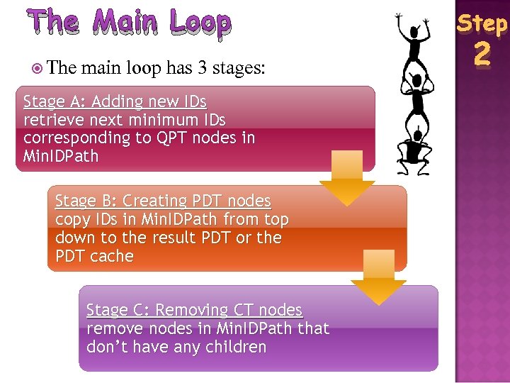 The Main Loop The main loop has 3 stages: Stage A: Adding new IDs retrieve next minimum IDs corresponding to QPT nodes in Min. IDPath Stage B: Creating PDT nodes copy IDs in Min. IDPath from top down to the result PDT or the PDT cache Stage C: Removing CT nodes remove nodes in Min. IDPath that don’t have any children Step 2
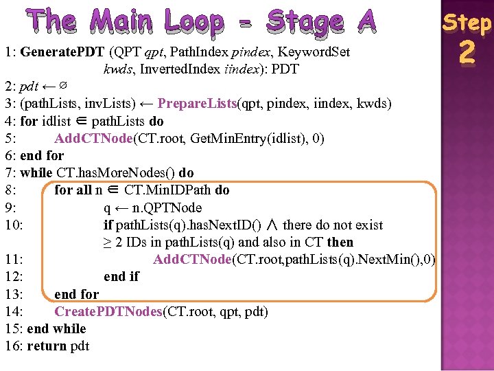 The Main Loop - Stage A 1: Generate. PDT (QPT qpt, Path. Index pindex, Keyword. Set kwds, Inverted. Index iindex): PDT 2: pdt ← ∅ 3: (path. Lists, inv. Lists) ← Prepare. Lists(qpt, pindex, iindex, kwds) 4: for idlist ∈ path. Lists do 5: Add. CTNode(CT. root, Get. Min. Entry(idlist), 0) 6: end for 7: while CT. has. More. Nodes() do 8: for all n ∈ CT. Min. IDPath do 9: q ← n. QPTNode 10: if path. Lists(q). has. Next. ID() ∧ there do not exist ≥ 2 IDs in path. Lists(q) and also in CT then 11: Add. CTNode(CT. root, path. Lists(q). Next. Min(), 0) 12: end if 13: end for 14: Create. PDTNodes(CT. root, qpt, pdt) 15: end while 16: return pdt Step 2
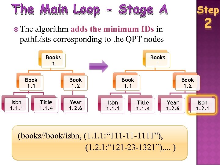 The Main Loop - Stage A Step 2 The algorithm adds the minimum IDs in path. Lists corresponding to the QPT nodes Books 1 Book 1. 1 Isbn 1. 1. 1 Book 1. 2 Title 1. 1. 4 Year 1. 2. 6 (books//book/isbn, (1. 1. 1: “ 111 -11 -1111”), (1. 2. 1: “ 121 -23 -1321”), . . . ) Isbn 1. 2. 1
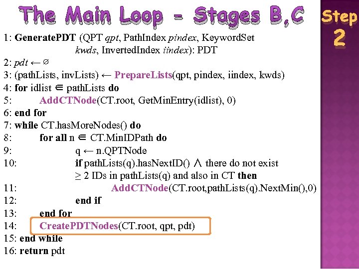 The Main Loop - Stages B, C 1: Generate. PDT (QPT qpt, Path. Index pindex, Keyword. Set kwds, Inverted. Index iindex): PDT 2: pdt ← ∅ 3: (path. Lists, inv. Lists) ← Prepare. Lists(qpt, pindex, iindex, kwds) 4: for idlist ∈ path. Lists do 5: Add. CTNode(CT. root, Get. Min. Entry(idlist), 0) 6: end for 7: while CT. has. More. Nodes() do 8: for all n ∈ CT. Min. IDPath do 9: q ← n. QPTNode 10: if path. Lists(q). has. Next. ID() ∧ there do not exist ≥ 2 IDs in path. Lists(q) and also in CT then 11: Add. CTNode(CT. root, path. Lists(q). Next. Min(), 0) 12: end if 13: end for 14: Create. PDTNodes(CT. root, qpt, pdt) 15: end while 16: return pdt Step 2
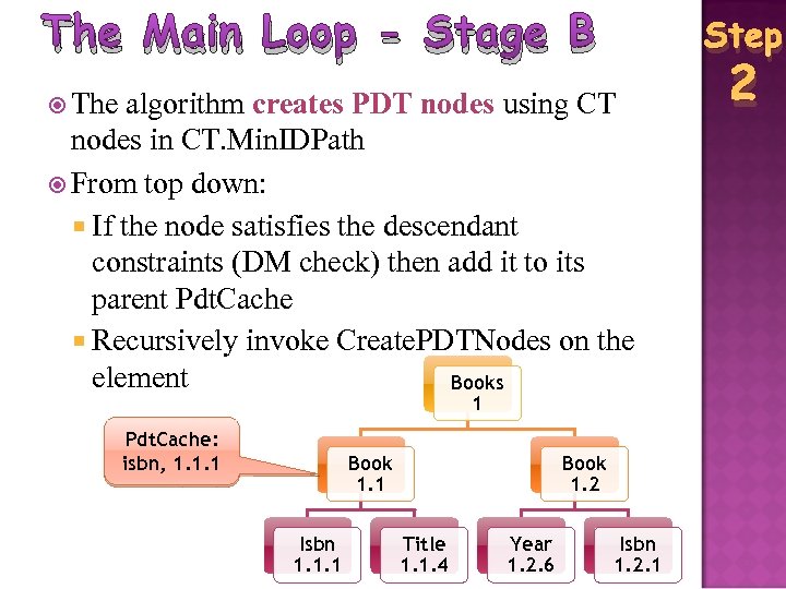 The Main Loop - Stage B Step The algorithm creates PDT nodes using CT nodes in CT. Min. IDPath From top down: If the node satisfies the descendant constraints (DM check) then add it to its parent Pdt. Cache Recursively invoke Create. PDTNodes on the element Books 1 Pdt. Cache: isbn, 1. 1. 1 Book 1. 1 Isbn 1. 1. 1 Book 1. 2 Title 1. 1. 4 Year 1. 2. 6 Isbn 1. 2. 1 2
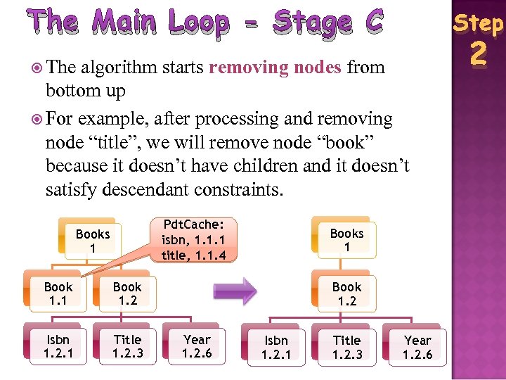 The Main Loop - Stage C Step The algorithm starts removing nodes from bottom up For example, after processing and removing node “title”, we will remove node “book” because it doesn’t have children and it doesn’t satisfy descendant constraints. Pdt. Cache: isbn, 1. 1. 1 title, 1. 1. 4 Books 1 Book 1. 2 Isbn 1. 2. 1 Title 1. 2. 3 Books 1 Book 1. 2 Year 1. 2. 6 Isbn 1. 2. 1 Title 1. 2. 3 Year 1. 2. 6 2
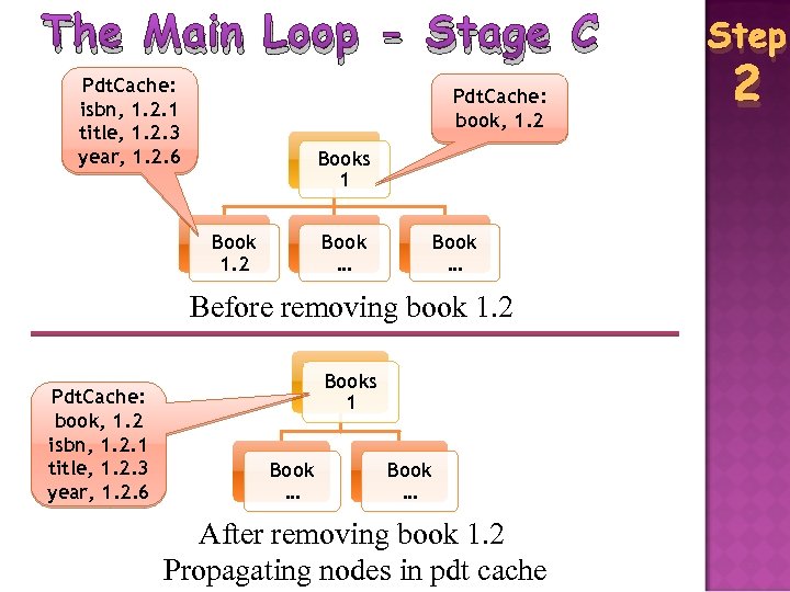 The Main Loop - Stage C Pdt. Cache: isbn, 1. 2. 1 title, 1. 2. 3 year, 1. 2. 6 Pdt. Cache: book, 1. 2 Books 1 Book 1. 2 Book … Before removing book 1. 2 Pdt. Cache: book, 1. 2 isbn, 1. 2. 1 title, 1. 2. 3 year, 1. 2. 6 Books 1 Book … After removing book 1. 2 Propagating nodes in pdt cache Step 2
 The Main Loop - Stage C Since nodes are processed in id order, a node’s descendant constraints will never be satisfied in the future Next, we check if nodes satisfy ancestor constraints, which is done by checking nodes in their parent lists. If those parent nodes are known to be non-PDT nodes, then we can conclude that the nodes in the cache will not satisfy ancestor restrictions, and can hence be removed. Otherwise the cache node still has other parents, which could be PDT nodes, and will thus be propagated to the Pdt. Cache of the ancestor. Step 2
 Query Evaluation Once the PDTs are generated, they are fed to a traditional evaluator to produce the temporary results, which are then sent to the Scoring & Materialization Module. tf values are encoded as XML attributes tf-idf scores are calculated for each PDT element using tf values The Scoring & Materialization Module then identifies the view results with top-k scores. The contents of these results are retrieved from the document storage system Step 3
 Outline Motivation and Problem Definition Existing Data and Data Structures Algorithm Experiments
 Experiments


