T Tests and ANovas Jennifer Siegel Objectives

T Tests and ANovas Jennifer Siegel

Objectives Statistical background Z-Test T-Test Anovas

Predicting the Future from a Sample Science tries to predict the future Genuine effect? Attempt to strengthen predictions with stats Use P-Value to indicate our level of certainty that result = genuine effect on whole population (more on this later…)

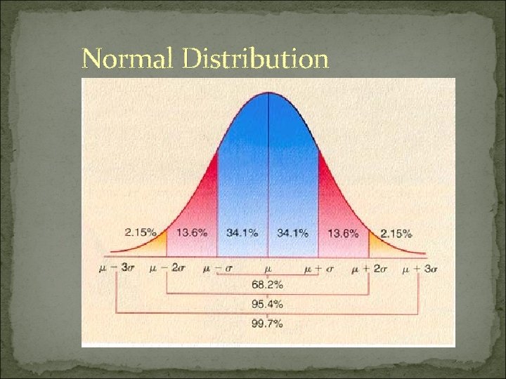
Normal Distribution

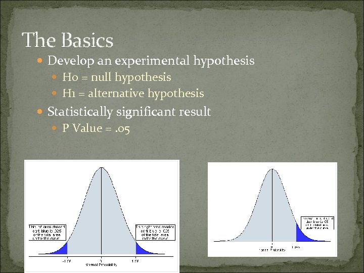
The Basics Develop an experimental hypothesis H 0 = null hypothesis H 1 = alternative hypothesis Statistically significant result P Value =. 05

P-Value Probability that observed result is true Level =. 05 or 5% 95% certain our experimental effect is genuine

Errors! Type 1 = false positive Type 2 = false negative P = 1 – Probability of Type 1 error

Research Question Example Let’s pretend you came up with the following theory… Having a baby increases brain volume (associated with possible structural changes)

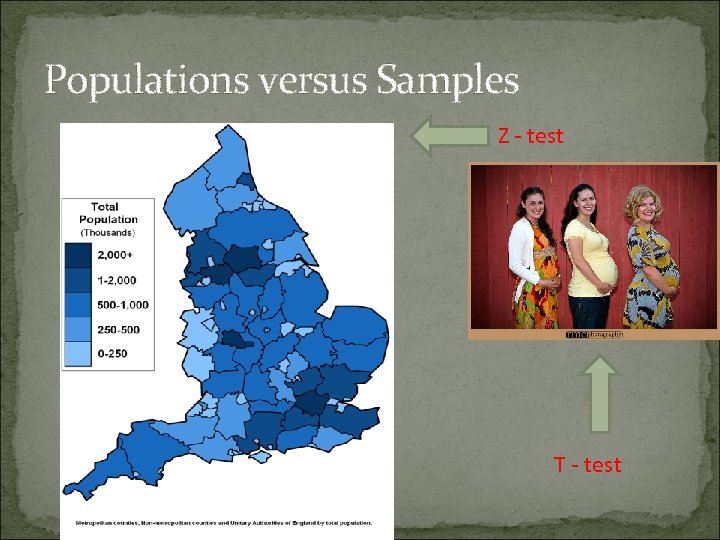
Populations versus Samples Z - test T - test

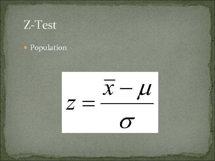
Z-Test Population

Some Problems with a Population-Based Study Cost Not able to include everyone Too time consuming Ethical right to privacy Realistically researchers can only do sample based studies

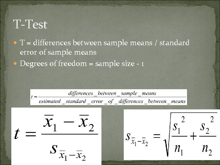
T-Test T = differences between sample means / standard error of sample means Degrees of freedom = sample size - 1

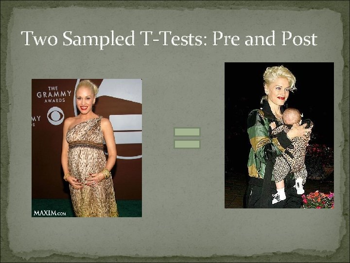
Two Sampled T-Tests: Pre and Post

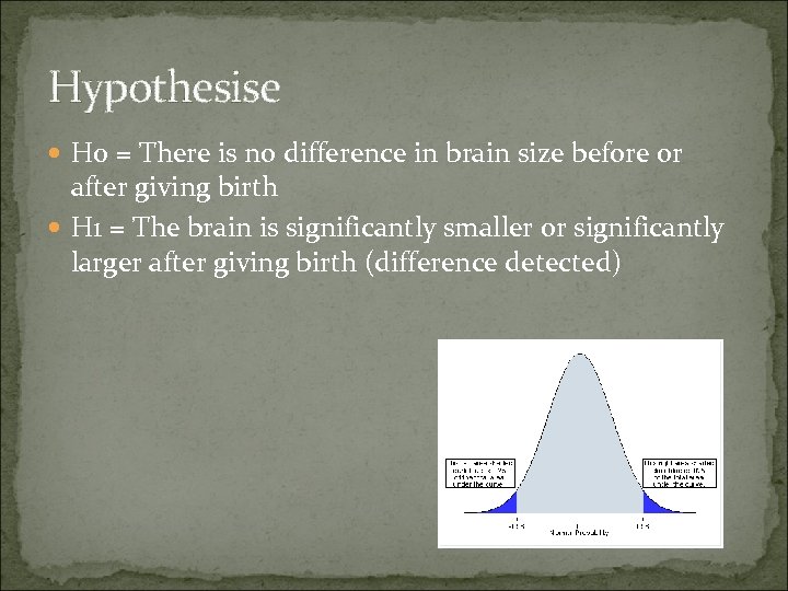
Hypothesise H 0 = There is no difference in brain size before or after giving birth H 1 = The brain is significantly smaller or significantly larger after giving birth (difference detected)

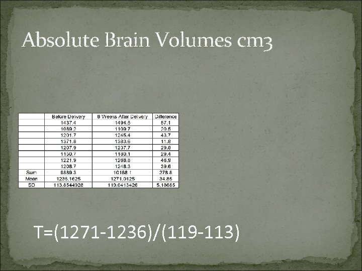
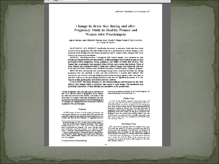
Absolute Brain Volumes cm 3 T=(1271 -1236)/(119 -113)

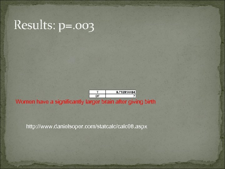
Results: p=. 003 Women have a significantly larger brain after giving birth http: //www. danielsoper. com/statcalc/calc 08. aspx

Types of T-Tests One-sample (sample vs. hypothesized mean) Independent groups (2 separate groups) Repeated measures (same group, different measure)

More than 1 group? ? ?

ANOVA ANalysis Of VAriance Factor = what is being compared (type of pregnancy) Levels = different elements of a factor (age of mother) F-Statistic Post hoc testing

Different types of Anova 1 Way Anova 1 factor with more than 2 levels Factorial Anova More than 1 factor Mixed Design Anovas Some factors are independent, others are related

What can be concluded from ANOVA There is a significant difference somewhere between groups NOT where the difference lies Finding exactly where the difference lies requires further statistical analysis = post hoc analysis

Conclusions Z-Tests for populations T-Tests for samples ANOVAS compare more than 2 groups in more complicated scenarios

Correlation and Linear Regression Varun V. Sethi

Objective Correlation Linear Regression Take Home Points.

With a few exceptions, every analysis is a variant of GLM

Correlation - How much linear is the relationship of two variables? (descriptive) Regression - How good is a linear model to explain my data? (inferential)

Correlation

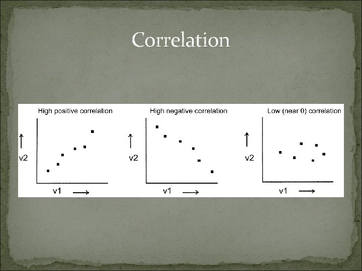
Correlation reflects the noisiness and direction of a linear relationship (top row), but not the slope of that relationship (middle), nor many aspects of nonlinear relationships (bottom).

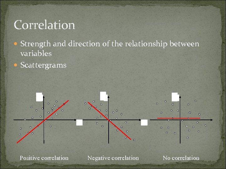
Correlation Strength and direction of the relationship between variables Scattergrams Y Y Y X Positive correlation Y Y Y X Negative correlation No correlation

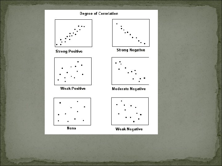
Measures of Correlation 1) Covariance 2) Pearson Correlation Coefficient (r)

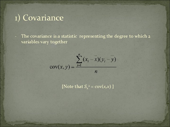
1) Covariance - The covariance is a statistic representing the degree to which 2 variables vary together {Note that Sx 2 = cov(x, x) }

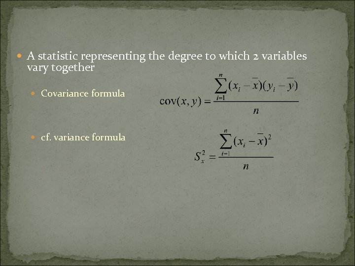
A statistic representing the degree to which 2 variables vary together Covariance formula cf. variance formula

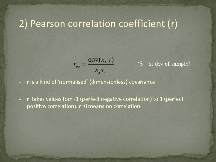
2) Pearson correlation coefficient (r) (S = st dev of sample) - r is a kind of ‘normalised’ (dimensionless) covariance - r takes values fom -1 (perfect negative correlation) to 1 (perfect positive correlation). r=0 means no correlation

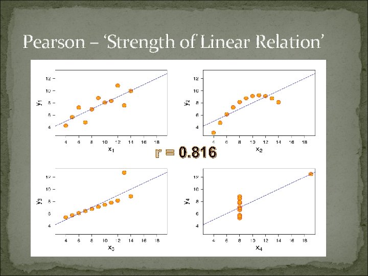
Pearson – ‘Strength of Linear Relation’ r = 0. 816

Limitations: Sensitive to extreme values Relationship not a prediction. Not Causality

Linear Regression

Regression: Prediction of one variable from knowledge of one or more other variables

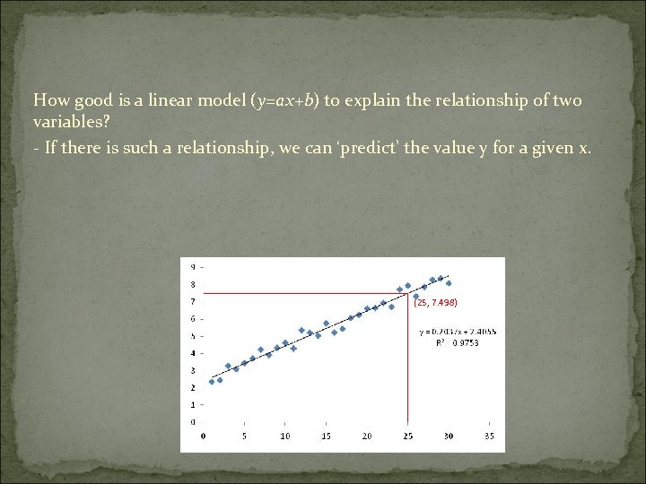
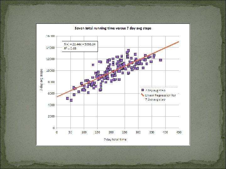
How good is a linear model (y=ax+b) to explain the relationship of two variables? - If there is such a relationship, we can ‘predict’ the value y for a given x. (25, 7. 498)

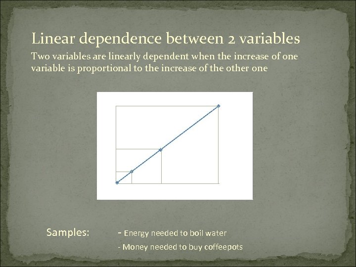
Linear dependence between 2 variables Two variables are linearly dependent when the increase of one variable is proportional to the increase of the other one y x Samples: - Energy needed to boil water - Money needed to buy coffeepots

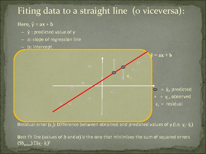
Fiting data to a straight line (o viceversa): Here, ŷ = ax + b – ŷ : predicted value of y – a: slope of regression line – b: intercept ŷ = ax + b εi = ŷi, predicted = yi , observed εi = residual Residual error (εi): Difference between obtained and predicted values of y (i. e. yi- ŷi) Best fit line (values of b and a) is the one that minimises the sum of squared errors (SSerror) (yi- ŷi)2

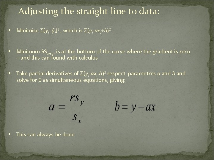
Adjusting the straight line to data: • Minimise (yi- ŷi)2 , which is (yi-axi+b)2 • Minimum SSerror is at the bottom of the curve where the gradient is zero – and this can found with calculus • Take partial derivatives of (yi-axi-b)2 respect parametres a and b and solve for 0 as simultaneous equations, giving: • This can always be done

How good is the model? We can calculate the regression line for any data, but how well does it fit the data? Total variance = predicted variance + error variance sy 2 = sŷ 2 + ser 2 Also, it can be shown that r 2 is the proportion of the variance in y that is explained by our regression model r 2 = s ŷ 2 / s y 2 Insert r 2 sy 2 into sy 2 = sŷ 2 + ser 2 and rearrange to get: ser 2 = sy 2 (1 – r 2) From this we can see that the greater the correlation the smaller the error variance, so the better our prediction

Is the model significant? Do we get a significantly better prediction of y from our regression equation than by just predicting the mean? F-statistic

Practical Uses of Linear Regression Prediction / Forecasting Quantify strength between y and Xj ( X 1, X 2, X 3 )

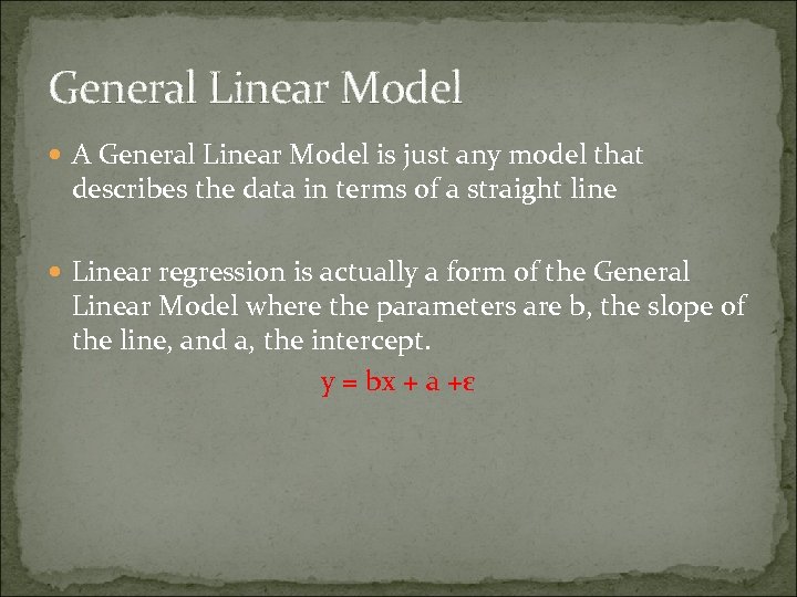
General Linear Model A General Linear Model is just any model that describes the data in terms of a straight line Linear regression is actually a form of the General Linear Model where the parameters are b, the slope of the line, and a, the intercept. y = bx + a +ε

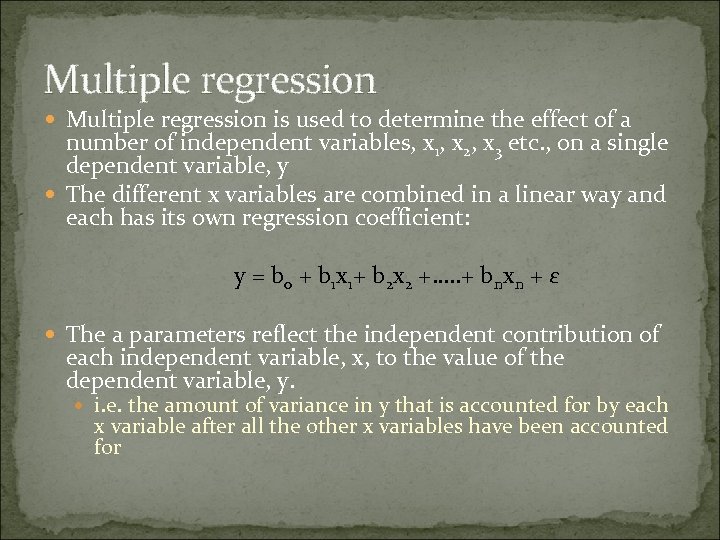
Multiple regression is used to determine the effect of a number of independent variables, x 1, x 2, x 3 etc. , on a single dependent variable, y The different x variables are combined in a linear way and each has its own regression coefficient: y = b 0 + b 1 x 1+ b 2 x 2 +…. . + bnxn + ε The a parameters reflect the independent contribution of each independent variable, x, to the value of the dependent variable, y. i. e. the amount of variance in y that is accounted for by each x variable after all the other x variables have been accounted for

Take Home Points - Correlated doesn’t mean related. e. g, any two variables increasing or decreasing over time would show a nice correlation: C 02 air concentration in Antartica and lodging rental cost in London. Beware in longitudinal studies!!! - Relationship between two variables doesn’t mean causality (e. g leaves on the forest floor and hours of sun)

Linear regression is a GLM that models the effect of one independent variable, x, on one dependent variable, y Multiple Regression models the effect of several independent variables, x 1, x 2 etc, on one dependent variable, y Both are types of General Linear Model

Thank You