870df5bf1da7448dcf94bb08044f2395.ppt
- Количество слайдов: 46
System Dynamics Simulation in Support of Obesity Prevention Decision-Making Bobby Milstein and Jack Homer For Institute of Medicine Committee on an Evidence Framework for Obesity Prevention Decision-Making Irvine, California March 16, 2009
Agenda v System Dynamics Background v Obesity Life-Course Model (2005 -2006, CDC) v Cardiovascular Risk Model (2007 -2010, CDC & NIH)
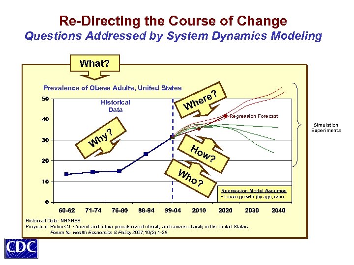
Re-Directing the Course of Change Questions Addressed by System Dynamics Modeling What? Prevalence of Obese Adults, United States Historical Data ? e her W Regression Forecast Simulation Experiments ? hy W Ho w ? Wh o? Regression Model Assumes • Linear growth (by age, sex) Historical Data: NHANES Projection: Ruhm CJ. Current and future prevalence of obesity and severe obesity in the United States. Forum for Health Economics & Policy 2007; 10(2): 1 -28.
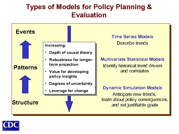
Types of Models for Policy Planning & Evaluation Events Increasing: Time Series Models Describe trends • Depth of causal theory Patterns • Robustness for longerterm projection • Value for developing policy insights • Degrees of uncertainty • Leverage for change Structure Multivariate Statistical Models Identify historical trend drivers and correlates Dynamic Simulation Models Anticipate new trends, learn about policy consequences, and set justifiable goals
System Dynamics Simulating Dynamic Complexity Origins • Jay Forrester, MIT, Industrial Dynamics, 1961 (“One of the seminal books of the last 20 years. ”-- NY Times) • Public policy applications starting late 1960 s • Population health applications starting mid 1970 s Good at Capturing • Differences between short- and long-term consequences of an action • Time delays (e. g. , incubation period, time to detect, time to respond) • Accumulations (e. g. , prevalences, resources, attitudes) • Behavioral feedback (reactions by various actors) • Nonlinear causal relationships (e. g. , threshold effects, saturation effects) • Differences or inconsistencies in goals/values among stakeholders Forrester JW. Industrial Dynamics. Cambridge, MA: MIT Press; 1961. Sterman JD. Business Dynamics: Systems Thinking and Modeling for a Complex World. Boston, MA: Irwin/Mc. Graw-Hill; 2000.
System Dynamics Health Applications 1970 s to the Present • Disease epidemiology – Cardiovascular, diabetes, obesity, HIV/AIDS, cervical cancer, chlamydia, dengue fever, drugresistant infections • Substance abuse epidemiology – Heroin, cocaine, tobacco • Health care patient flows – Acute care, long-term care • Health care capacity and delivery – Managed care, dental care, mental health care, disaster preparedness, community health programs • Health system economics – Interactions of providers, payers, patients, and investors Homer J, Hirsch G. System dynamics modeling for public health: Background and opportunities. American Journal of Public Health 2006; 96(3): 452 -458.
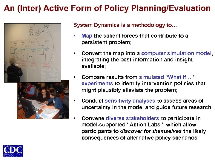
An (Inter) Active Form of Policy Planning/Evaluation System Dynamics is a methodology to… • Map the salient forces that contribute to a persistent problem; • Convert the map into a computer simulation model, integrating the best information and insight available; • Compare results from simulated “What If…” experiments to identify intervention policies that might plausibly alleviate the problem; • Conduct sensitivity analyses to assess areas of uncertainty in the model and guide future research; • Convene diverse stakeholders to participate in model-supported “Action Labs, ” which allow participants to discover for themselves the likely consequences of alternative policy scenarios
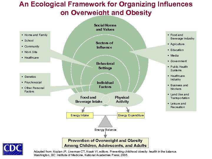
An Ecological Framework for Organizing Influences on Overweight and Obesity Social Norms and Values § Home and Family § Food and Beverage Industry § School Sectors of Influence § Community § Agriculture § Education § Work Site § Media § Healthcare § Government Behavioral Settings § Public Health Systems § Healthcare Industry § Genetics § Psychosocial Individual Factors § Other Personal Factors Food and Beverage Intake § Business and Workers Physical Activity Energy Intake § Land Use and Transportation § Leisure and Recreation Energy Expenditure Energy Balance Prevention of Overweight and Obesity Among Children, Adolescents, and Adults Adapted from: Koplan JP, Liverman CT, Kraak VI, editors. Preventing childhood obesity: health in the balance. Washington, DC: Institute of Medicine, National Academies Press; 2005.
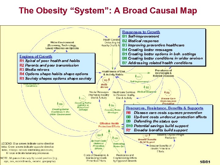
The Obesity “System”: A Broad Causal Map Engines of Growth R 1 Spiral of poor health and habits R 2 Parents and peer transmission R 3 Media mirrors R 4 Options shape habits shape options R 5 Society shapes options shape society Responses to Growth B 1 Self-improvement B 2 Medical response B 3 Improving preventive healthcare B 4 Creating better messages B 5 Creating better options in beh. settings B 6 Creating better conditions in wider environ B 7 Addressing related health conditions Resources, Resistance, Benefits & Supports R 6 Disease care costs squeeze prevention B 8 Up-front costs undercut protection efforts B 9 Defending the status quo B 10 Potential savings build support R 7 Broader benefits build support 5/8/05
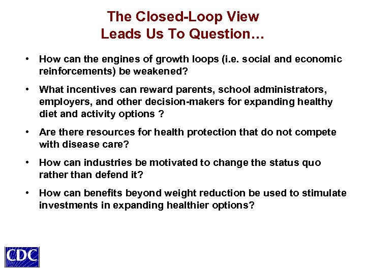
The Closed-Loop View Leads Us To Question… • How can the engines of growth loops (i. e. social and economic reinforcements) be weakened? • What incentives can reward parents, school administrators, employers, and other decision-makers for expanding healthy diet and activity options ? • Are there resources for health protection that do not compete with disease care? • How can industries be motivated to change the status quo rather than defend it? • How can benefits beyond weight reduction be used to stimulate investments in expanding healthier options?
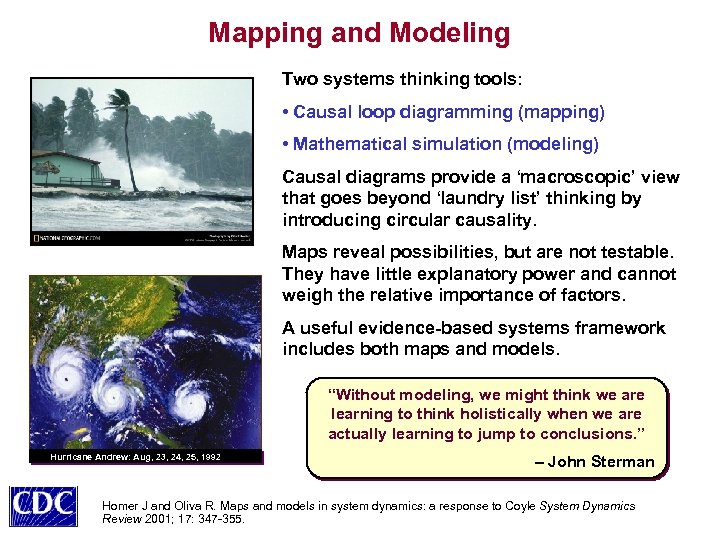
Mapping and Modeling Two systems thinking tools: • Causal loop diagramming (mapping) • Mathematical simulation (modeling) Causal diagrams provide a ‘macroscopic’ view that goes beyond ‘laundry list’ thinking by introducing circular causality. Maps reveal possibilities, but are not testable. They have little explanatory power and cannot weigh the relative importance of factors. A useful evidence-based systems framework includes both maps and models. “Without modeling, we might think we are learning to think holistically when we are actually learning to jump to conclusions. ” Hurricane Andrew: Aug, 23, 24, 25, 1992 – John Sterman Homer J and Oliva R. Maps and models in system dynamics: a response to Coyle System Dynamics Review 2001; 17: 347 -355.
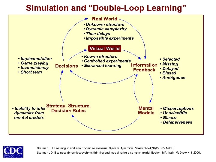
Simulation and “Double-Loop Learning” Real World • Unknown structure • Dynamic complexity • Time delays • Impossible experiments Virtual World • Known structure • Implementation • Controlled experiments • Game playing Information Decisions • Enhanced learning • Inconsistency Feedback • Short term • Inability to infer Strategy, Structure, Decision Rules dynamics from mental models Mental Models • Selected • Missing • Delayed • Biased • Ambiguous • Misperceptions • Unscientific • Biases • Defensiveness Sterman JD. Learning in and about complex systems. System Dynamics Review 1994; 10(2 -3): 291 -330. Sterman JD. Business dynamics: systems thinking and modeling for a complex world. Boston, MA: Irwin Mc. Graw-Hill, 2000.
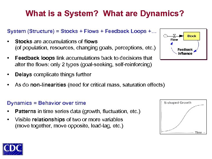
What is a System? What are Dynamics? System (Structure) = Stocks + Flows + Feedback Loops +… • Stocks are accumulations of flows (of population, resources, changing goals, perceptions, etc. ) • Feedback loops link accumulations back to decisions that alter the flows: only 2 types (goal-seeking, self-reinforcing) • Delays complicate things further • As do non-linearities (need for critical mass, saturation effects) Dynamics = Behavior over time • Patterns in time series data (growth, fluctuation, etc. ) • Visible relationships of two or more variables (move together, move opposite, lead-lag, etc. )
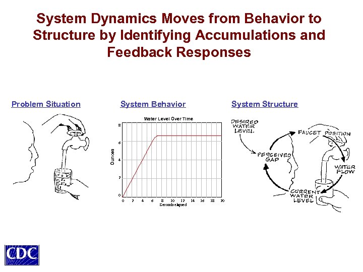
System Dynamics Moves from Behavior to Structure by Identifying Accumulations and Feedback Responses Problem Situation System Behavior System Structure Water Level Over Time 8 Ounces 6 4 2 0 0 2 4 6 8 10 12 14 Seconds elapsed 16 18 20
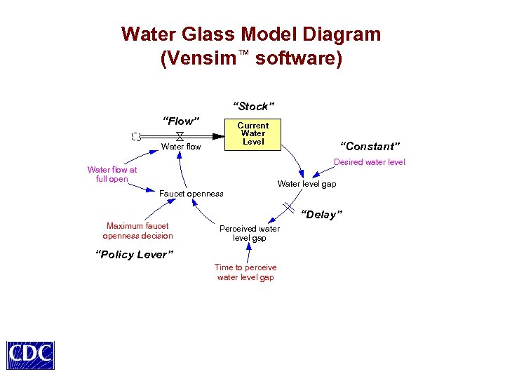
Water Glass Model Diagram (Vensim™ software) “Stock” “Flow” Current Water Level Water flow “Constant” Desired water level Water flow at full open Water level gap Faucet openness “Delay” Maximum faucet openness decision Perceived water level gap “Policy Lever” Time to perceive water level gap
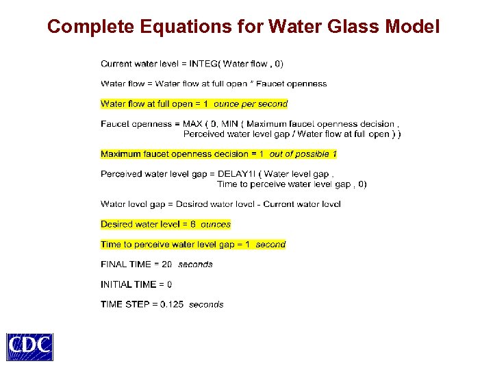
Complete Equations for Water Glass Model
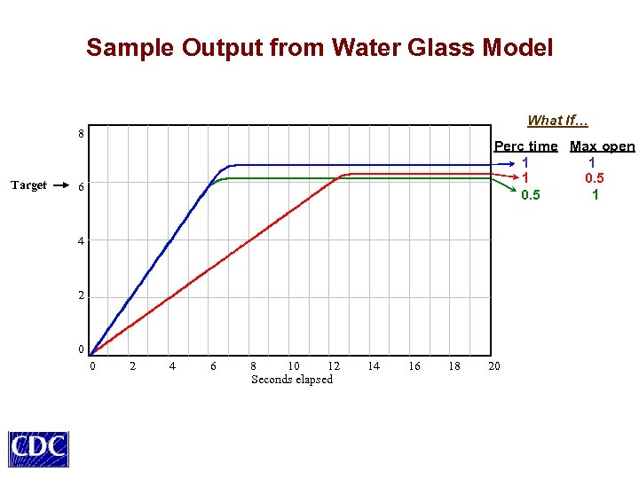
Sample Output from Water Glass Model What If… 8 Target Ounces Perc time Max open 1 1 1 0. 5 1 6 4 2 0 0 2 4 6 8 10 12 Seconds elapsed 14 16 18 20
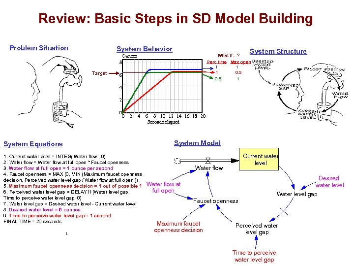
Review: Basic Steps in SD Model Building Problem Situation System Behavior System Structure What if…? Perc time Max open 1 1 1 0. 5 1 Ounces 8 Target 6 4 2 0 0 2 4 System Equations 1. Current water level = INTEG( Water flow , 0) 2. Water flow = Water flow at full open * Faucet openness 3. Water flow at full open = 1 ounce per second 4. Faucet openness = MAX (0, MIN (Maximum faucet openness decision, Perceived water level gap / Water flow at full open )) 5. Maximum faucet openness decision = 1 out of possible 1 6. Perceived water level gap = DELAY 1 I (Water level gap, Time to perceive water level gap, 0) 7. Water level gap = Desired water level - Current water level 8. Desired water level = 6 ounces 9. Time to perceive water level gap = 1 second FINAL TIME = 20 seconds INITIAL TIME = 0 TIME STEP = 0. 125 seconds 6 8 10 12 14 16 18 20 Seconds elapsed System Model Current water level Water flow Desired water level Water level gap Water flow at full open Faucet openness Maximum faucet openness decision Perceived water level gap Time to perceive water level gap
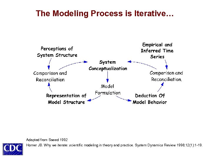
The Modeling Process is Iterative… Adapted from Saeed 1992 Homer JB. Why we iterate: scientific modeling in theory and practice. System Dynamics Review 1996; 12(1): 1 -19.
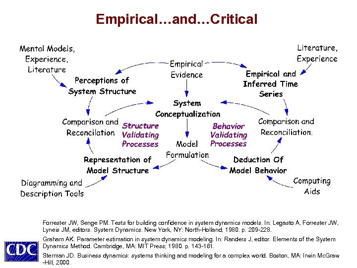
Empirical…and…Critical Forrester JW, Senge PM. Tests for building confidence in system dynamics models. In: Legasto A, Forrester JW, Lyneis JM, editors. System Dynamics. New York, NY: North-Holland; 1980. p. 209 -228. Graham AK. Parameter estimation in system dynamics modeling. In: Randers J, editor. Elements of the System Dynamics Method. Cambridge, MA: MIT Press; 1980. p. 143 -161. Sterman JD. Business dynamics: systems thinking and modeling for a complex world. Boston, MA: Irwin Mc. Graw -Hill, 2000.
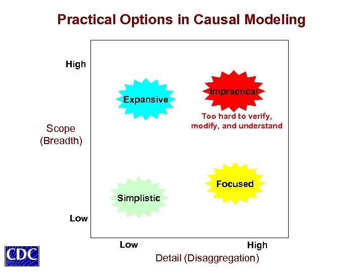
Practical Options in Causal Modeling High Expansive Impractical Too hard to verify, modify, and understand Scope (Breadth) Focused Simplistic Low High Detail (Disaggregation)
Model Structure and Level of Detail Depends on the Intended Uses and Audiences • Set Better Goals (Planners & Evaluators) – Identify what is likely and what is possible – Estimate intervention impact time profiles – Evaluate resource needs for meeting goals • Support Better Action (Policymakers) – Explore ways of combining policies for better results – Evaluate cost-effectiveness over extended time periods – Increase policymakers’ motivation to act differently • Develop Better Theory and Estimates (Researchers) – – Integrate and reconcile diverse data sources Identify causal mechanisms driving system behavior Improve estimates of hard-to-measure or “hidden” variables Identify key uncertainties to address in intervention studies Forrester JW. Industrial Dynamics (Chapter 11: Aggregation of Variables). Cambridge, MA: MIT Press, 1961.
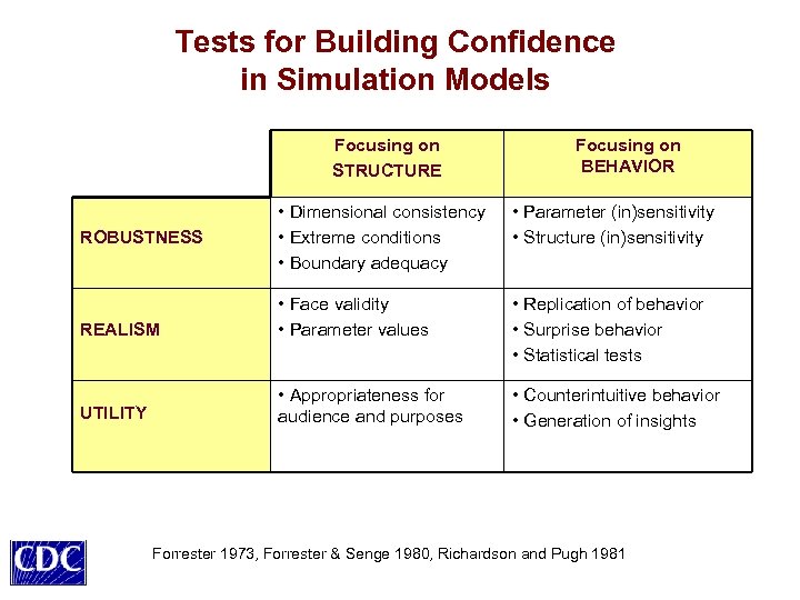
Tests for Building Confidence in Simulation Models Focusing on STRUCTURE Focusing on BEHAVIOR • Dimensional consistency • Extreme conditions • Boundary adequacy • Parameter (in)sensitivity • Structure (in)sensitivity REALISM • Face validity • Parameter values • Replication of behavior • Surprise behavior • Statistical tests UTILITY • Appropriateness for audience and purposes • Counterintuitive behavior • Generation of insights ROBUSTNESS Forrester 1973, Forrester & Senge 1980, Richardson and Pugh 1981
The Future of Systems Simulation • More ambitious models, addressing big strategic questions • Supporting macro-models with more empirical data, but also with the results of focused (operational, mechanistic) micro-models • Improved use of expert judgment; e. g. , Delphi method • More use of software tools for automated model calibration, sensitivity testing, and documentation • Better public outreach through logical, balanced presentation that provides clear path from evidence to insight “There seems to be a common attitude that the major difficulty is shortage of information and data. Once data are collected, people feel confident in interpreting the implications. I differ on both of these attitudes. The problem is not shortage of data but rather our inability to perceive the consequences of the information we already possess. ” – Jay Forrester JW. System dynamics—the next fifty years. System Dynamics Review 2007; 23(2/3): 345 -358. Homer JB. Macro- and micro-modeling of field service dynamics. System Dynamics Review 1999; 15(2): 139 -162. Meadows DH, Robinson JM. The Electronic Oracle: Computer Models and Social Decisions. Wiley & Sons, 1985.
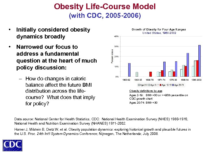
Obesity Life-Course Model (with CDC, 2005 -2006) • Initially considered obesity dynamics broadly Growth of Obesity for Four Age Ranges United States, 1960 -2002 • Narrowed our focus to address a fundamental question at the heart of much policy discussion: – How do changes in caloric balance affect the future BMI distribution across the lifecourse? What does that imply for policy? Obesity definitions by age Ages 2 -19: BMI>=30 or >=95 th percentile on CDC growth chart Ages 20 -74: BMI>=30 Data source: National Center for Health Statistics, CDC: National Health Examination Survey (NHES) 1960 -1970, National Health and Nutrition Examination Survey (NHANES) 1971 -2002. Homer J, Milstein B, Dietz W, et al. Obesity population dynamics: exploring historical growth and plausible futures in the U. S. Proc. 24 th Int’l System Dynamics Conference; Nijmegen, The Netherlands; July 2006.
Focusing on Life-Course Dynamics • Explore likely consequences of possible interventions affecting caloric balance (intake less expenditure) – How much impact on obesity prevalence? – How long will it take to see? – Should we target particular subpopulations? (age, sex, weight category; lack data for race, ethnicity) • Consider interventions broadly but leave details (composition, coverage, efficacy, cost) outside model boundary for now – Available data inadequate – Would require a separate research effort to estimate these details – Not addressing feedback loops of reinforcement and resistance – Not addressing cost-effectiveness
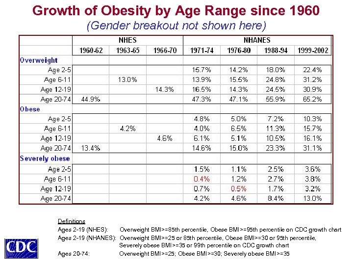
Growth of Obesity by Age Range since 1960 (Gender breakout not shown here) Definitions Ages 2 -19 (NHES): Overweight BMI>=85 th percentile, Obese BMI>=95 th percentile on CDC growth chart Ages 2 -19 (NHANES): Overweight BMI>=25 or 85 th percentile, Obese BMI>=30 or 95 th percentile, Severely obese BMI>=35 or 99 th percentile on CDC growth chart Ages 20 -74: Overweight BMI>=25; Obese BMI>=30; Severely obese BMI>=35
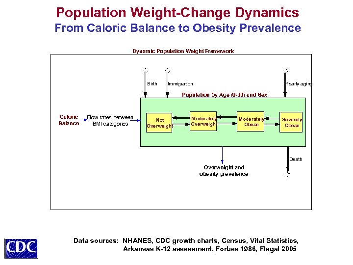
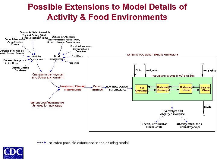
Population Weight-Change Dynamics From Caloric Balance to Obesity Prevalence Dynamic Population Weight Framework Birth Immigration Yearly aging Population by Age (0 -99) and Sex Caloric Balance Flow-rates between BMI categories Not Overweight Moderately Obese Severely Obese Death Overweight and obesity prevalence Data sources: NHANES, CDC growth charts, Census, Vital Statistics, Arkansas K-12 assessment, Forbes 1986, Flegal 2005
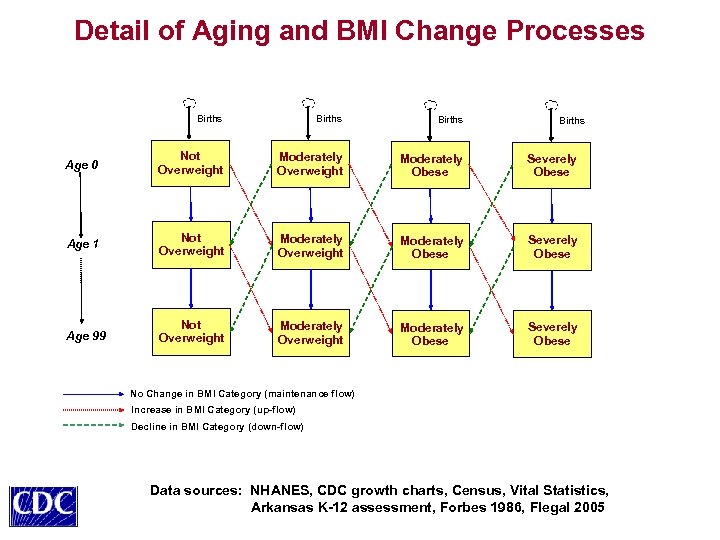
Detail of Aging and BMI Change Processes Births Age 0 Not Overweight Moderately Obese Severely Obese Age 1 Not Overweight Moderately Obese Severely Obese Age 99 Not Overweight Moderately Obese Severely Obese Births No Change in BMI Category (maintenance flow) Increase in BMI Category (up-flow) Decline in BMI Category (down-flow) Data sources: NHANES, CDC growth charts, Census, Vital Statistics, Arkansas K-12 assessment, Forbes 1986, Flegal 2005
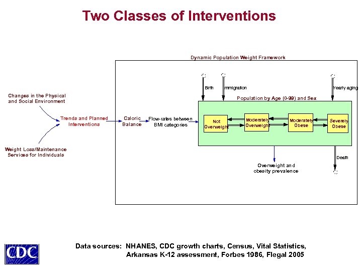
Two Classes of Interventions Dynamic Population Weight Framework Birth Immigration Changes in the Physical and Social Environment Yearly aging Population by Age (0 -99) and Sex Trends and Planned Interventions Caloric Balance Flow-rates between BMI categories Not Overweight Moderately Obese Weight Loss/Maintenance Services for Individuals Severely Obese Death Overweight and obesity prevalence Data sources: NHANES, CDC growth charts, Census, Vital Statistics, Arkansas K-12 assessment, Forbes 1986, Flegal 2005
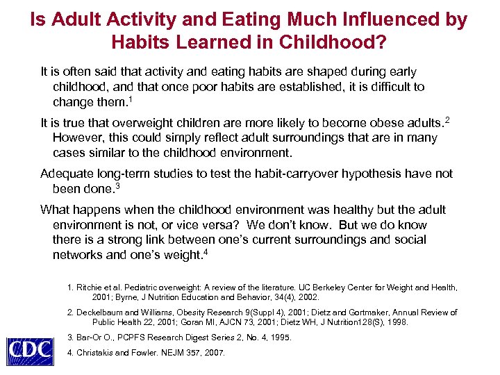
Is Adult Activity and Eating Much Influenced by Habits Learned in Childhood? It is often said that activity and eating habits are shaped during early childhood, and that once poor habits are established, it is difficult to change them. 1 It is true that overweight children are more likely to become obese adults. 2 However, this could simply reflect adult surroundings that are in many cases similar to the childhood environment. Adequate long-term studies to test the habit-carryover hypothesis have not been done. 3 What happens when the childhood environment was healthy but the adult environment is not, or vice versa? We don’t know. But we do know there is a strong link between one’s current surroundings and social networks and one’s weight. 4 1. Ritchie et al. Pediatric overweight: A review of the literature. UC Berkeley Center for Weight and Health, 2001; Byrne, J Nutrition Education and Behavior, 34(4), 2002. 2. Deckelbaum and Williams, Obesity Research 9(Suppl 4), 2001; Dietz and Gortmaker, Annual Review of Public Health 22, 2001; Goran MI, AJCN 73, 2001; Dietz WH, J Nutrition 128(S), 1998. 3. Bar-Or O. , PCPFS Research Digest Series 2, No. 4, 1995. 4. Christakis and Fowler. NEJM 357, 2007.
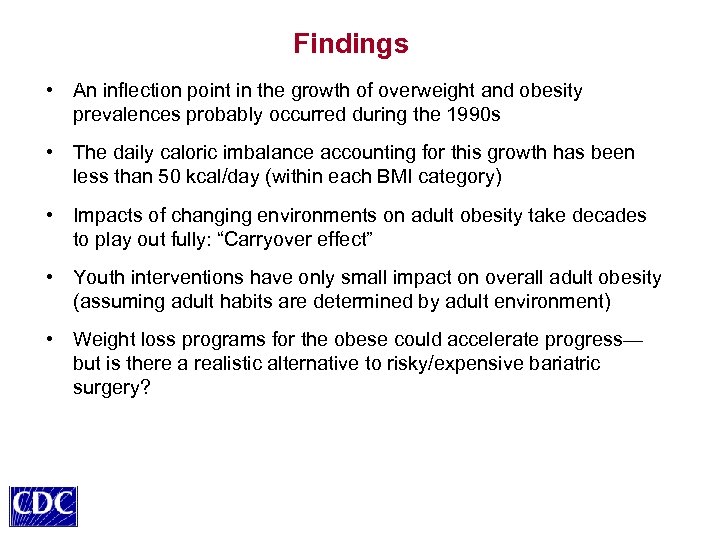
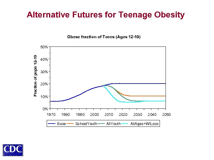
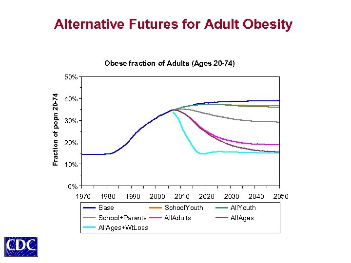
Findings • An inflection point in the growth of overweight and obesity prevalences probably occurred during the 1990 s • The daily caloric imbalance accounting for this growth has been less than 50 kcal/day (within each BMI category) • Impacts of changing environments on adult obesity take decades to play out fully: “Carryover effect” • Youth interventions have only small impact on overall adult obesity (assuming adult habits are determined by adult environment) • Weight loss programs for the obese could accelerate progress— but is there a realistic alternative to risky/expensive bariatric surgery?
Alternative Futures for Teenage Obesity Obese fraction of Teens (Ages 12 -19) Fraction of popn 12 -19 50% 40% 30% 20% 10% 0% 1970 1980 Base 1990 2000 School. Youth 2010 2020 All. Youth 2030 2040 All. Ages+Wt. Loss 2050
Alternative Futures for Adult Obesity Obese fraction of Adults (Ages 20 -74) Fraction of popn 20 -74 50% 40% 30% 20% 10% 0% 1970 1980 1990 Base School+Parents All. Ages+Wt. Loss 2000 2010 2020 School. Youth All. Adults 2030 2040 All. Youth All. Ages 2050
Possible Extensions to Model Details of Activity & Food Environments Options for Safe, Accessible Physical Activity (Work, Options for Affordable School, Neighborhoods) Social Influences on Recommended Foods (Work, Active/Inactive School, Markets, Restaurants) Options Social Influences on Consumption & Distance from Home to Selection Work, School, Errands Food Price Food Activity Environment Electronic Media Smoking in the Home Dynamic Population Weight Framework Activity Limiting Conditions Birth Immigration Changes in the Physical and Social Environment Trends and Planned Interventions Yearly aging Population by Age (0 -99) and Sex Caloric Balance Flow-rates between BMI categories Not Overweight Moderately Obese Severely Obese Weight Loss/Maintenance Services for Individuals Death Overweight and obesity prevalence Obesity-attributable illness costs Indicates possible extensions to the existing model Obesity-attributable unhealthy days
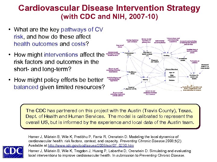
Cardiovascular Disease Intervention Strategy (with CDC and NIH, 2007 -10) • What are the key pathways of CV risk, and how do these affect health outcomes and costs? • How might interventions affect the risk factors and outcomes in the short- and long-term? • How might policy efforts be better balanced given limited resources? The CDC has partnered on this project with the Austin (Travis County), Texas, Dept. of Health and Human Services. The model is calibrated to represent the overall US, but is informed by the experience and local data of the Austin team. Homer J, Milstein B, Wile K, Pratibhu P, Farris R, Orenstein D. Modeling the local dynamics of cardiovascular health: risk factors, context, and capacity. Preventing Chronic Disease 2008; 5(2). Available at http: //www. cdc. gov/pcd/issues/2008/apr/07_0230. htm Homer J, Milstein B, Wile K, Trogdon J, Huang P, Labarthe D, Orenstein D. Simulating and evaluating local interventions to improve cardiovascular health. In submission to Preventing Chronic Disease.
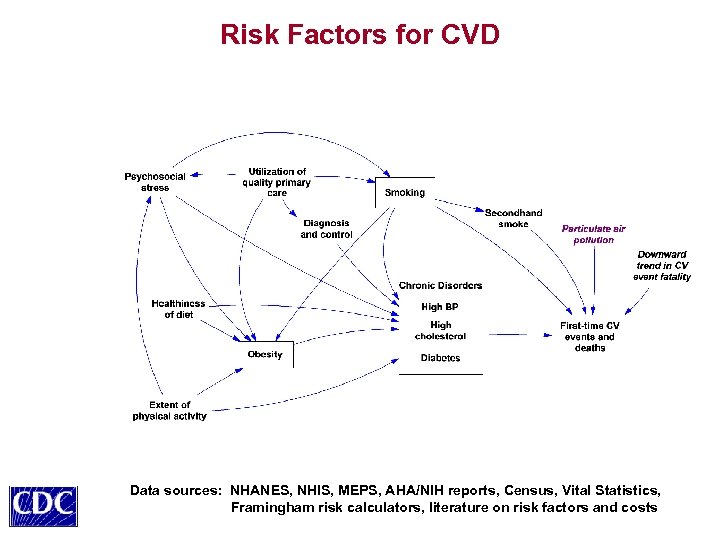
Risk Factors for CVD Data sources: NHANES, NHIS, MEPS, AHA/NIH reports, Census, Vital Statistics, Framingham risk calculators, literature on risk factors and costs
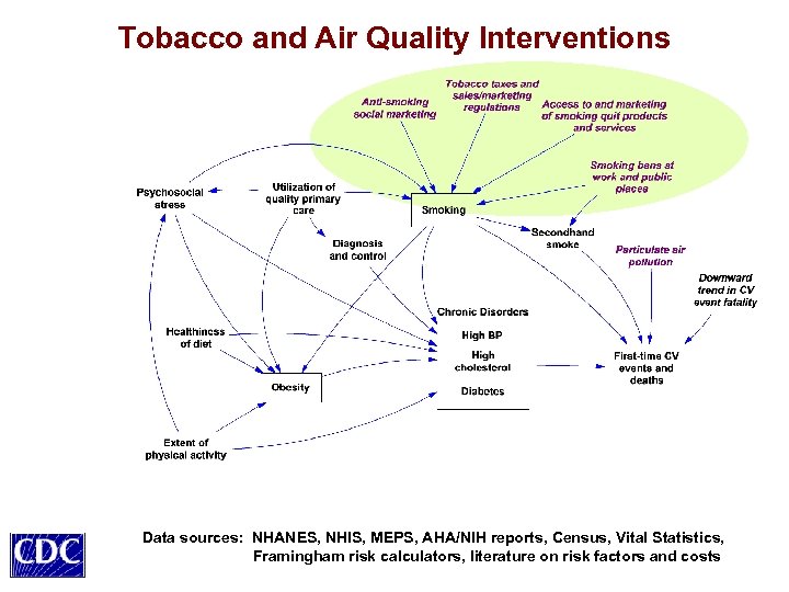
Tobacco and Air Quality Interventions Data sources: NHANES, NHIS, MEPS, AHA/NIH reports, Census, Vital Statistics, Framingham risk calculators, literature on risk factors and costs
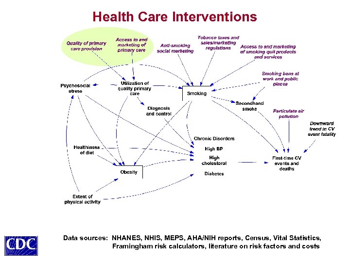
Health Care Interventions Data sources: NHANES, NHIS, MEPS, AHA/NIH reports, Census, Vital Statistics, Framingham risk calculators, literature on risk factors and costs
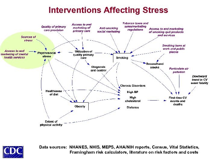
Interventions Affecting Stress Data sources: NHANES, NHIS, MEPS, AHA/NIH reports, Census, Vital Statistics, Framingham risk calculators, literature on risk factors and costs
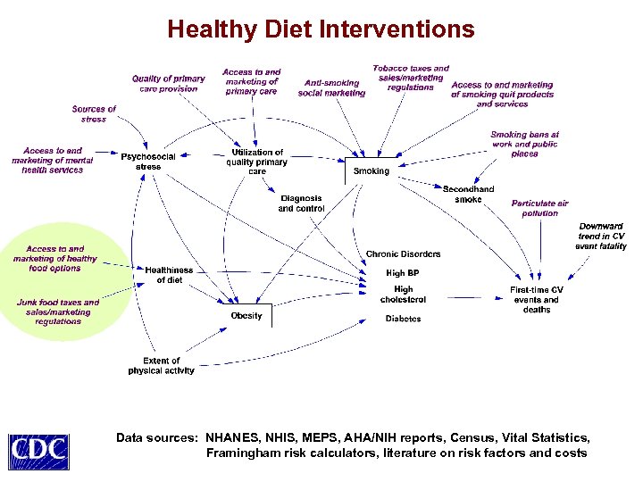
Healthy Diet Interventions Data sources: NHANES, NHIS, MEPS, AHA/NIH reports, Census, Vital Statistics, Framingham risk calculators, literature on risk factors and costs
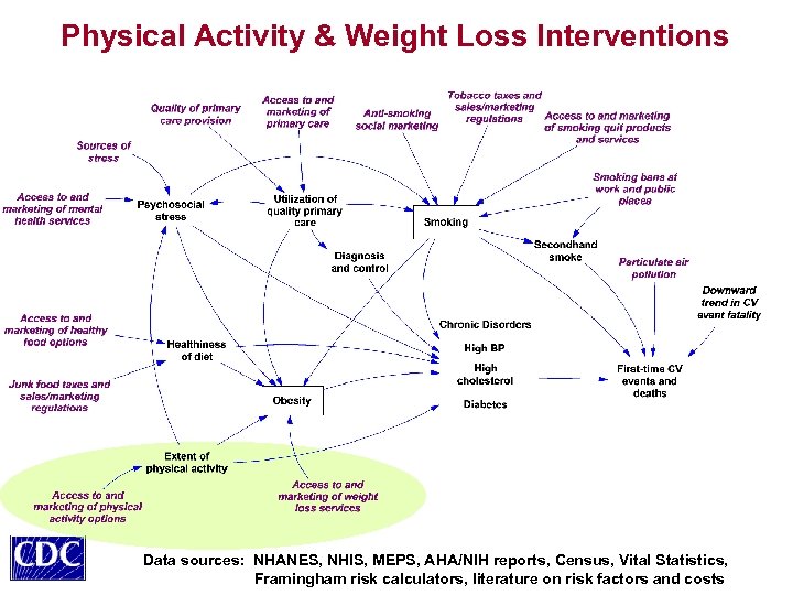
Physical Activity & Weight Loss Interventions Data sources: NHANES, NHIS, MEPS, AHA/NIH reports, Census, Vital Statistics, Framingham risk calculators, literature on risk factors and costs
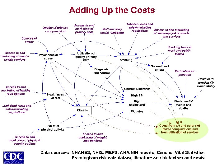
Adding Up the Costs Data sources: NHANES, NHIS, MEPS, AHA/NIH reports, Census, Vital Statistics, Framingham risk calculators, literature on risk factors and costs
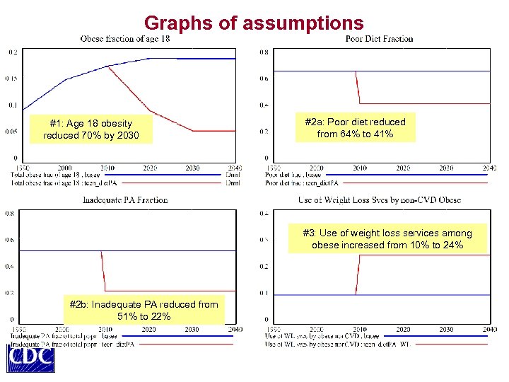
Graphs of assumptions #1: Age 18 obesity reduced 70% by 2030 #2 a: Poor diet reduced from 64% to 41% #3: Use of weight loss services among obese increased from 10% to 24% #2 b: Inadequate PA reduced from 51% to 22%
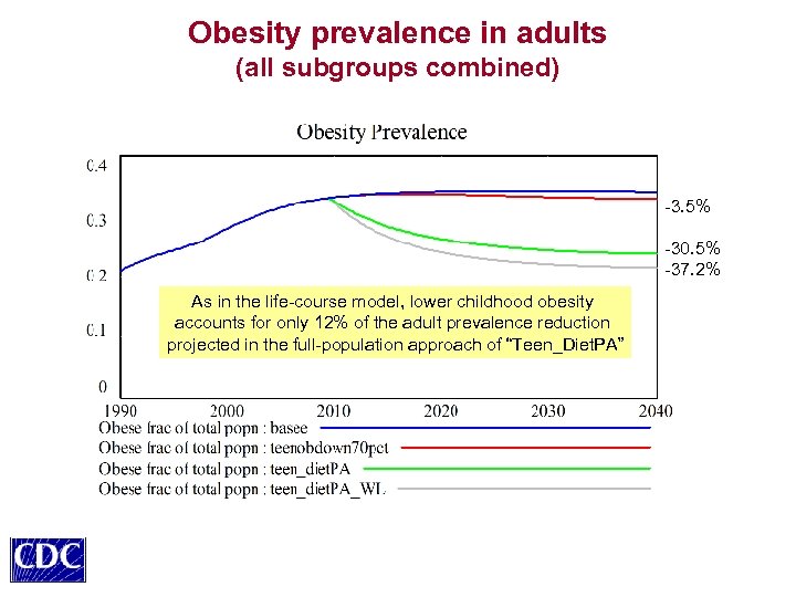
Obesity prevalence in adults (all subgroups combined) -3. 5% -30. 5% -37. 2% As in the life-course model, lower childhood obesity accounts for only 12% of the adult prevalence reduction projected in the full-population approach of “Teen_Diet. PA”
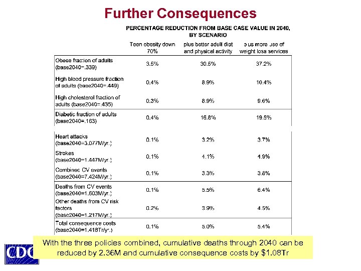
Further Consequences With the three policies combined, cumulative deaths through 2040 can be reduced by 2. 36 M and cumulative consequence costs by $1. 08 Tr
870df5bf1da7448dcf94bb08044f2395.ppt