589c9e635a247de5d55b261af12b073a.ppt
- Количество слайдов: 65
Surface-based Group Analysis in Free. Surfer
Outline • Group Analysis Overview • Theory • Surface-based Intersubject Registration • Surface-based Smoothing • General Linear Model (GLM) • Practice • FSGD File • Processing Stages • Vertex-wise Analysis • Correction for multiple comparisons • Interactive/Automated GUI (QDEC) 2
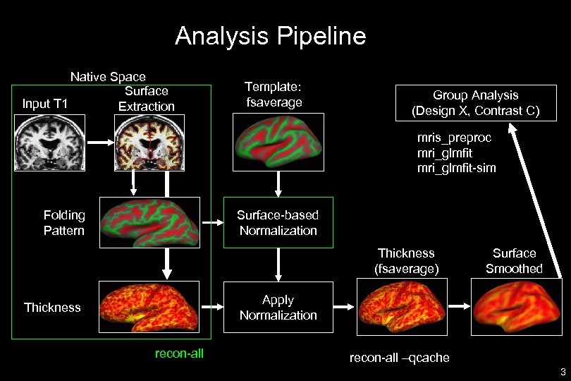
Analysis Pipeline Native Space Surface Input T 1 Extraction Template: fsaverage Group Analysis (Design X, Contrast C) mris_preproc mri_glmfit-sim Folding Pattern Surface-based Normalization Thickness (fsaverage) Surface Smoothed Apply Normalization Thickness recon-all –qcache 3
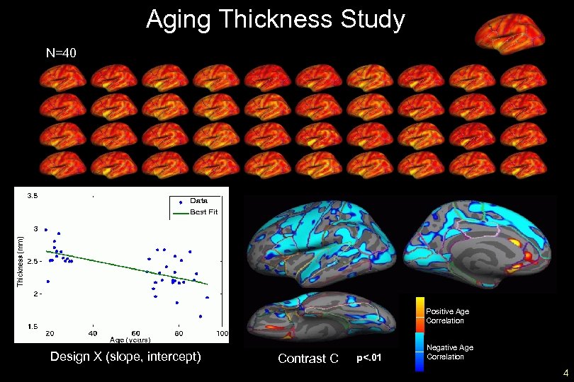
Aging Thickness Study N=40 Positive Age Correlation Design X (slope, intercept) Contrast C p<. 01 Negative Age Correlation 4
Theory 1. Surface-based Intersubject Registration 2. Surface-based Smoothing 3. General Linear Model (GLM) 5
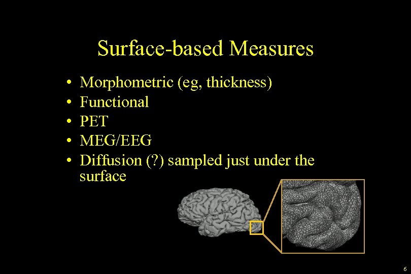
Surface-based Measures • • • Morphometric (eg, thickness) Functional PET MEG/EEG Diffusion (? ) sampled just under the surface 6
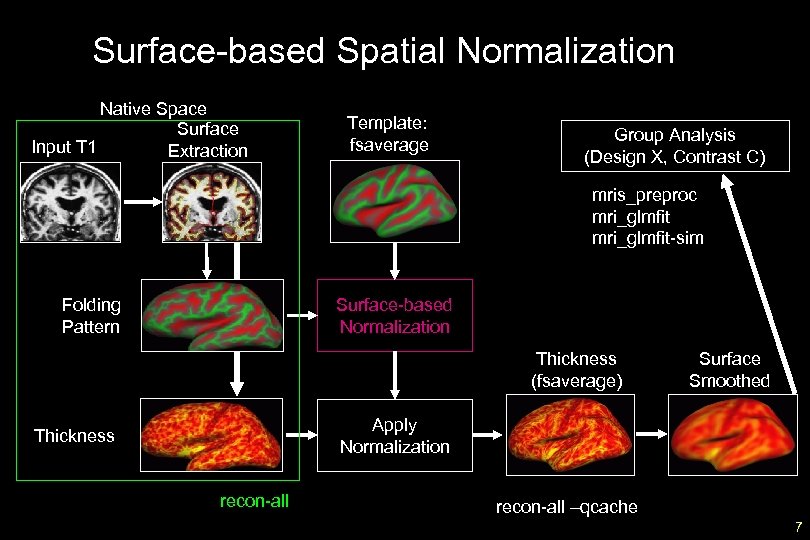
Surface-based Spatial Normalization Native Space Surface Input T 1 Extraction Template: fsaverage Group Analysis (Design X, Contrast C) mris_preproc mri_glmfit-sim Folding Pattern Surface-based Normalization Thickness (fsaverage) Surface Smoothed Apply Normalization Thickness recon-all –qcache 7
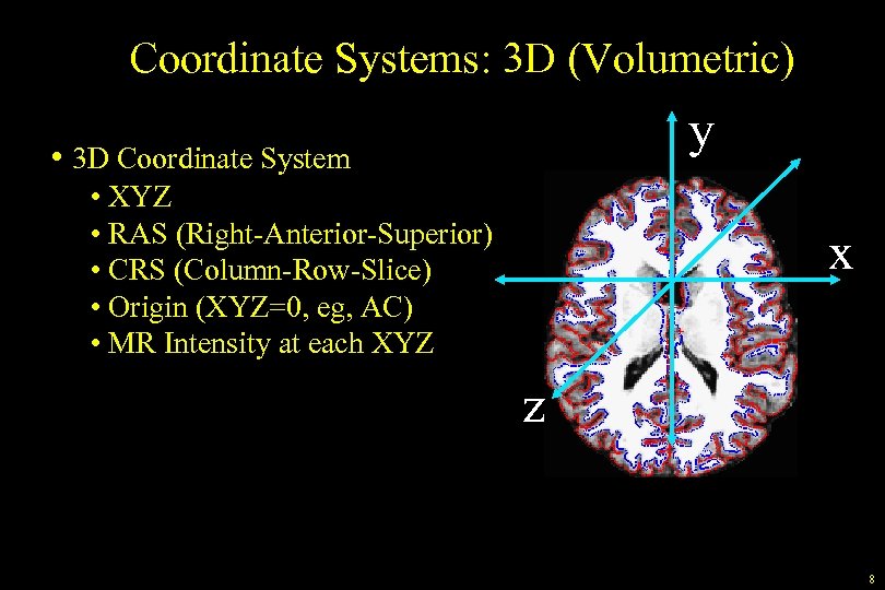
Coordinate Systems: 3 D (Volumetric) y • 3 D Coordinate System • XYZ • RAS (Right-Anterior-Superior) • CRS (Column-Row-Slice) • Origin (XYZ=0, eg, AC) • MR Intensity at each XYZ x z 8
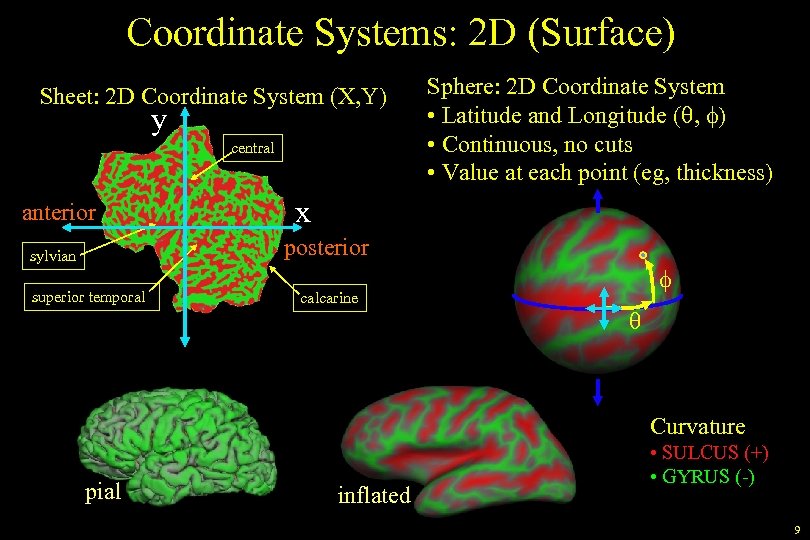
Coordinate Systems: 2 D (Surface) Sheet: 2 D Coordinate System (X, Y) y central anterior Sphere: 2 D Coordinate System • Latitude and Longitude (q, f) • Continuous, no cuts • Value at each point (eg, thickness) x posterior sylvian superior temporal calcarine f q Curvature pial inflated • SULCUS (+) • GYRUS (-) 9
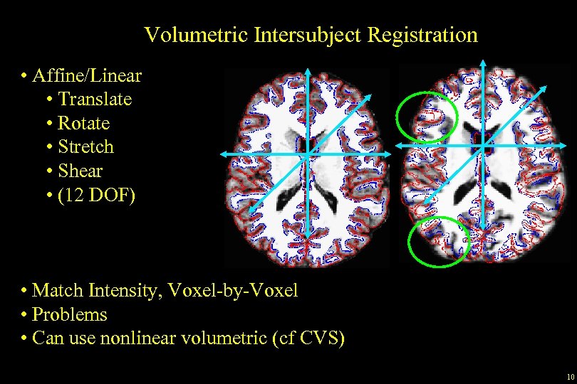
Volumetric Intersubject Registration • Affine/Linear • Translate • Rotate • Stretch • Shear • (12 DOF) • Match Intensity, Voxel-by-Voxel • Problems • Can use nonlinear volumetric (cf CVS) 10
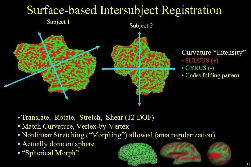
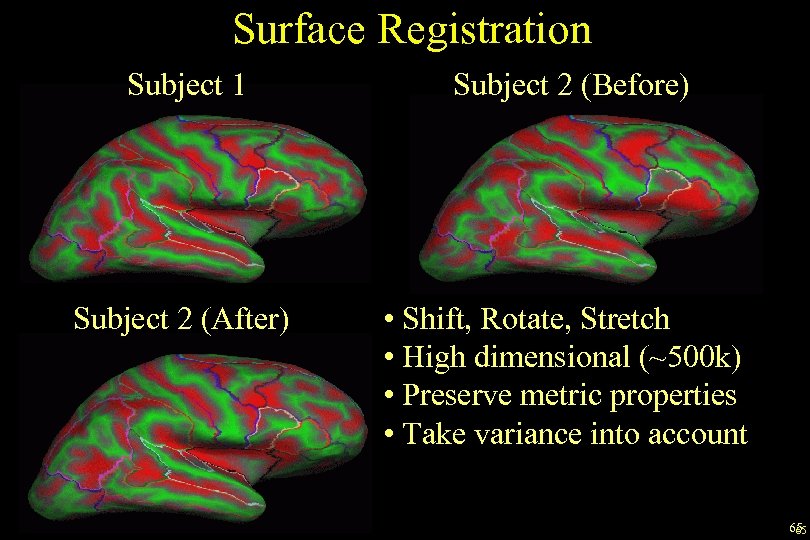
Surface-based Intersubject Registration Subject 1 Subject 2 Curvature “Intensity” • SULCUS (+) • GYRUS (-) • Codes folding pattern • Translate, Rotate, Stretch, Shear (12 DOF) • Match Curvature, Vertex-by-Vertex • Nonlinear Stretching (“Morphing”) allowed (area regularization) • Actually done on sphere • “Spherical Morph” 11
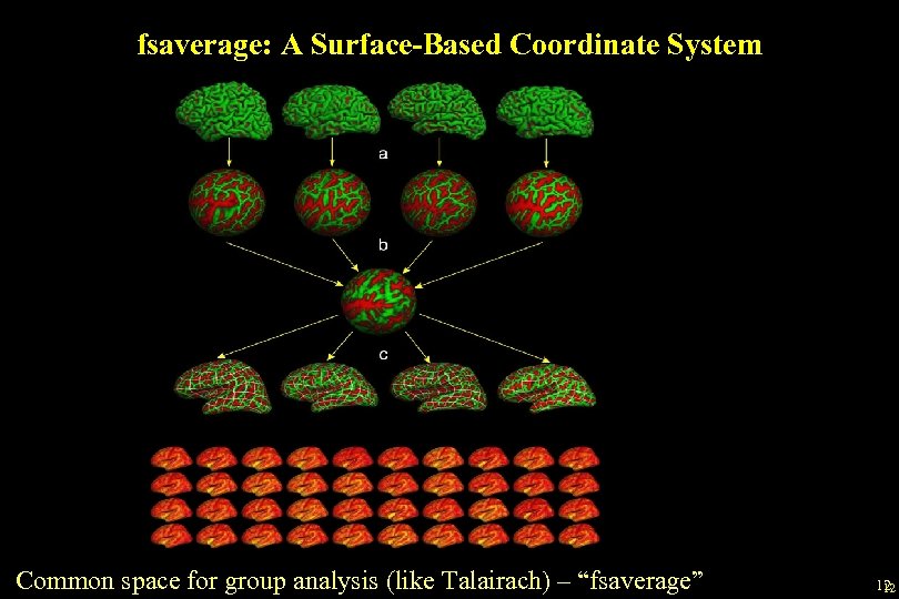
fsaverage: A Surface-Based Coordinate System Common space for group analysis (like Talairach) – “fsaverage” 12 12
Surface-based Intersubject Registration • Gray Matter-to-Gray Matter (it’s all gray matter!) • Gyrus-to-Gyrus and Sulcus-to-Sulcus • Some minor folding patterns won’t line up • Fully automated, no landmarking needed • Atlas registration is probabilistic, most variable regions get less weight. • Done automatically in recon-all 13
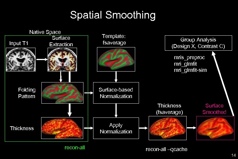
Spatial Smoothing Native Space Surface Input T 1 Extraction Template: fsaverage Group Analysis (Design X, Contrast C) mris_preproc mri_glmfit-sim Folding Pattern Surface-based Normalization Thickness (fsaverage) Surface Smoothed Apply Normalization Thickness recon-all –qcache 14
Spatial Smoothing Why should you smooth? • Might Improve CNR • Improve intersubject registration (functional) How much smoothing? • Blob-size • Typically 10 -20 mm FWHM • Surface smoothing more forgiving than volume-based 15
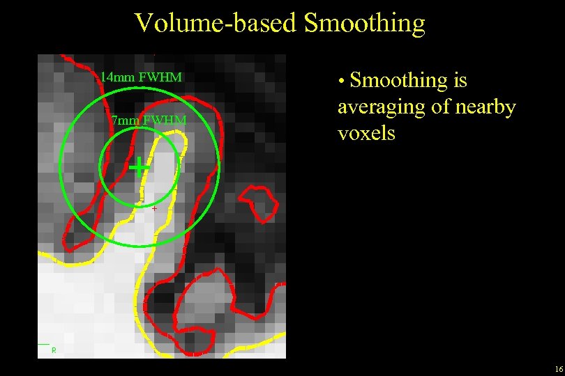
Volume-based Smoothing 14 mm FWHM 7 mm FWHM • Smoothing is averaging of nearby voxels 16
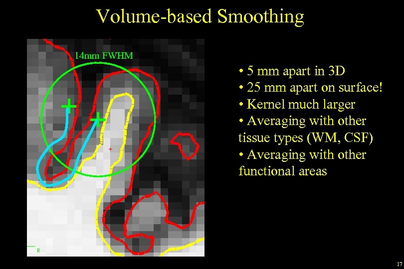
Volume-based Smoothing 14 mm FWHM • 5 mm apart in 3 D • 25 mm apart on surface! • Kernel much larger • Averaging with other tissue types (WM, CSF) • Averaging with other functional areas 17
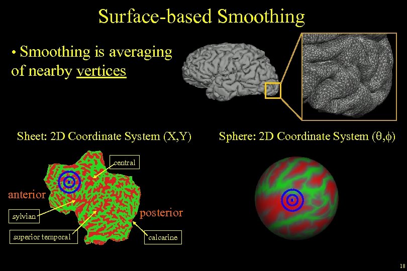
Surface-based Smoothing • Smoothing is averaging of nearby vertices Sheet: 2 D Coordinate System (X, Y) Sphere: 2 D Coordinate System (q, f) central anterior sylvian superior temporal posterior calcarine 18
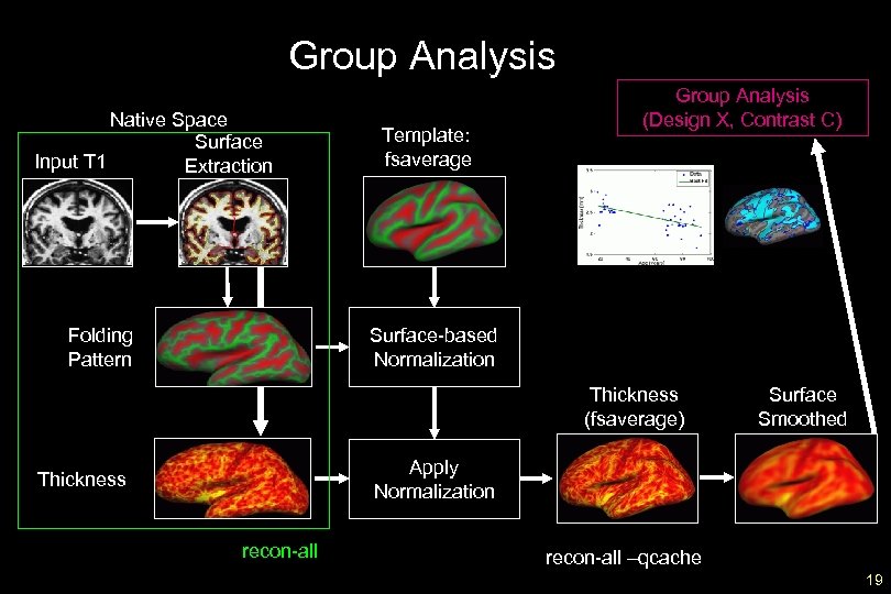
Group Analysis Native Space Surface Input T 1 Extraction Folding Pattern Template: fsaverage Group Analysis (Design X, Contrast C) Surface-based Normalization Thickness (fsaverage) Surface Smoothed Apply Normalization Thickness recon-all –qcache 19
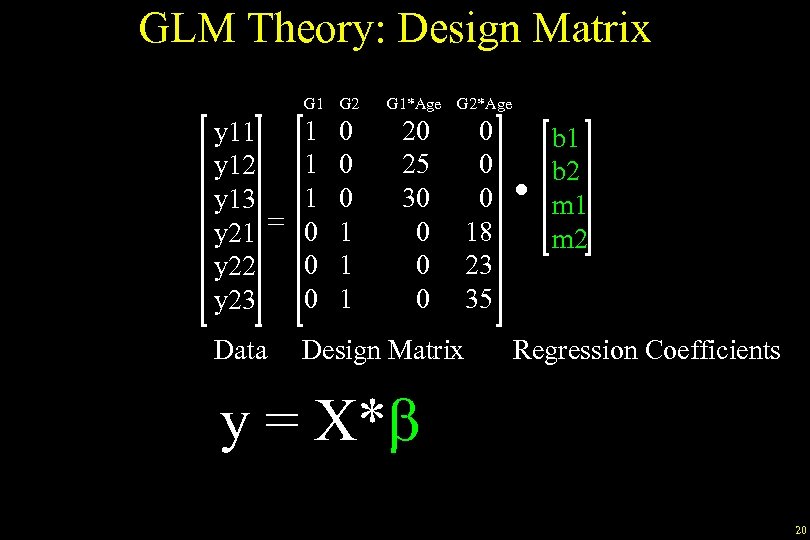
GLM Theory: Design Matrix G 1 G 2 1 0 y 11 1 0 y 12 1 0 y 13 y 21 = 0 1 y 22 0 1 y 23 Data G 1*Age G 2*Age 20 25 30 0 Design Matrix 0 0 0 18 23 35 . b 1 b 2 m 1 m 2 Regression Coefficients y = X*b 20
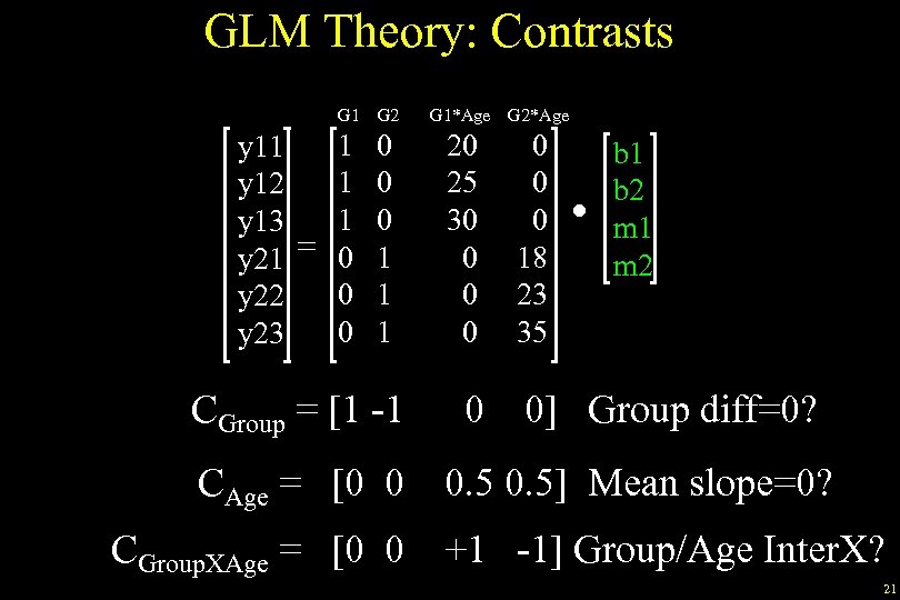
GLM Theory: Contrasts G 1 G 2 1 0 y 11 1 0 y 12 1 0 y 13 y 21 = 0 1 y 22 0 1 y 23 CGroup = [1 -1 CAge = [0 0 CGroup. XAge = [0 0 G 1*Age 20 25 30 0 0 G 2*Age 0 0 0 18 23 35 . b 1 b 2 m 1 m 2 0] Group diff=0? 0. 5] Mean slope=0? +1 -1] Group/Age Inter. X? 21
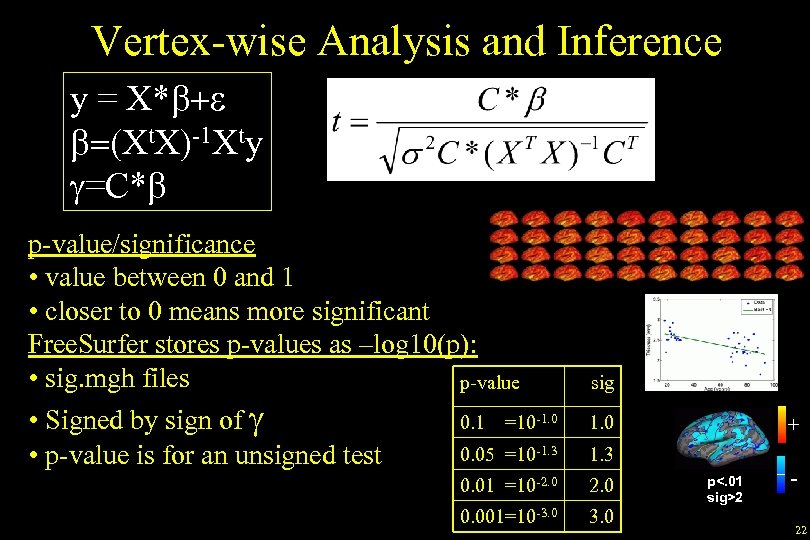
Vertex-wise Analysis and Inference y = X*b+e b=(Xt. X)-1 Xty g=C*b p-value/significance • value between 0 and 1 • closer to 0 means more significant Free. Surfer stores p-values as –log 10(p): • sig. mgh files p-value • Signed by sign of g • p-value is for an unsigned test 0. 1 sig =10 -1. 0 0. 05 =10 -1. 3 0. 01 =10 -2. 0 0. 001=10 -3. 0 + p<. 01 sig>2 22
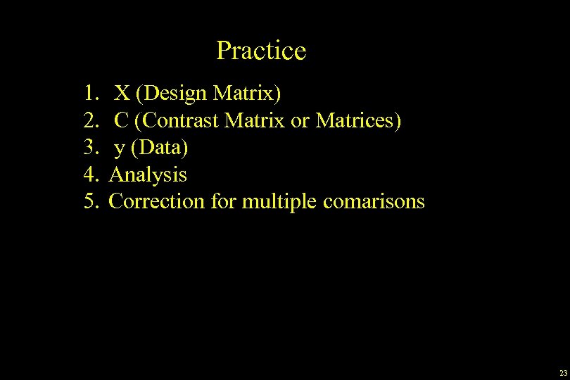
Practice 1. 2. 3. 4. 5. X (Design Matrix) C (Contrast Matrix or Matrices) y (Data) Analysis Correction for multiple comarisons 23
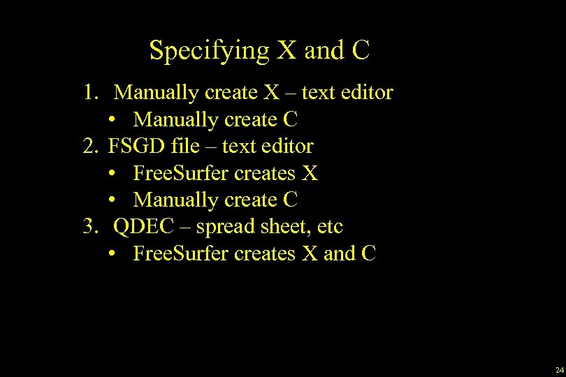
Specifying X and C 1. Manually create X – text editor • Manually create C 2. FSGD file – text editor • Free. Surfer creates X • Manually create C 3. QDEC – spread sheet, etc • Free. Surfer creates X and C 24
Free. Surfer Group Descriptor (FSGD) File • • Simple text file (ascii, clear text) List of all subjects in the study Accompanying demographics Like a spreadsheet 25
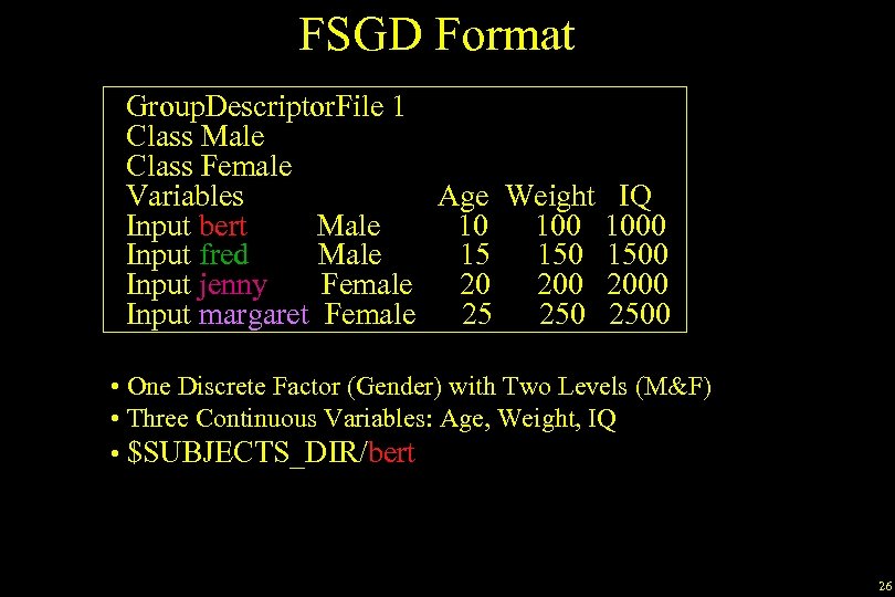
FSGD Format Group. Descriptor. File 1 Class Male Class Female Variables Age Weight IQ Input bert Male 10 1000 Input fred Male 15 1500 Input jenny Female 20 2000 Input margaret Female 25 2500 • One Discrete Factor (Gender) with Two Levels (M&F) • Three Continuous Variables: Age, Weight, IQ • $SUBJECTS_DIR/bert 26
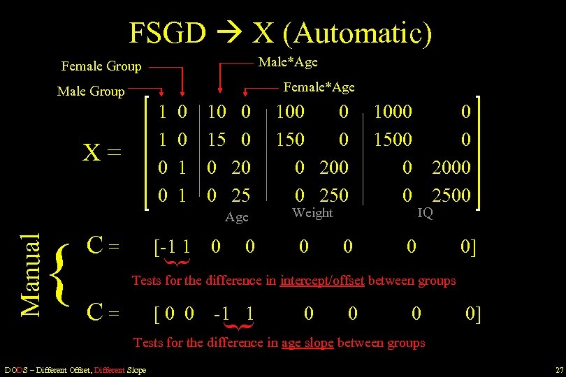
FSGD X (Automatic) Male*Age Female Group Female*Age Male Group 1 1 0 0 X= 0 0 1 1 10 0 15 0 0 25 Age Manual [-1 1 } { C= 0 0 100 0 150 0 0 200 0 250 Weight 0 0 1000 1500 0 0 2000 2500 IQ 0 0] Tests for the difference in intercept/offset between groups [0 0 -1 1 } C= 0 0] Tests for the difference in age slope between groups DODS – Different Offset, Different Slope 27
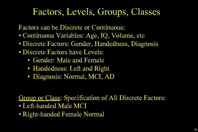
Factors, Levels, Groups, Classes Factors can be Discrete or Continuous: • Continuous Variables: Age, IQ, Volume, etc • Discrete Factors: Gender, Handedness, Diagnosis • Discrete Factors have Levels: • Gender: Male and Female • Handedness: Left and Right • Diagnosis: Normal, MCI, AD Group or Class: Specification of All Discrete Factors: • Left-handed Male MCI • Right-handed Female Normal 28
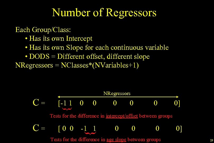
Number of Regressors Each Group/Class: • Has its own Intercept • Has its own Slope for each continuous variable • DODS = Different offset, different slope NRegressors = NClasses*(NVariables+1) NRegressors [-1 1 } C= 0 0 0] Tests for the difference in intercept/offset between groups [0 0 -1 1 } C= 0 0 0 Tests for the difference in age slope between groups 0] 29
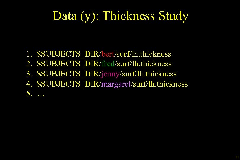
Data (y): Thickness Study 1. 2. 3. 4. 5. $SUBJECTS_DIR/bert/surf/lh. thickness $SUBJECTS_DIR/fred/surf/lh. thickness $SUBJECTS_DIR/jenny/surf/lh. thickness $SUBJECTS_DIR/margaret/surf/lh. thickness … 30
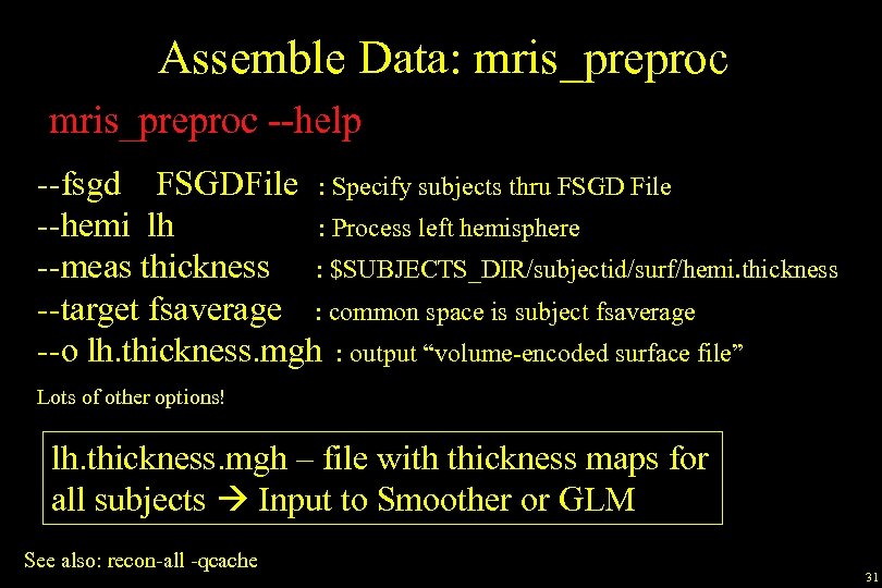
Assemble Data: mris_preproc --help --fsgd FSGDFile : Specify subjects thru FSGD File --hemi lh : Process left hemisphere --meas thickness : $SUBJECTS_DIR/subjectid/surf/hemi. thickness --target fsaverage : common space is subject fsaverage --o lh. thickness. mgh : output “volume-encoded surface file” Lots of other options! lh. thickness. mgh – file with thickness maps for all subjects Input to Smoother or GLM See also: recon-all -qcache 31
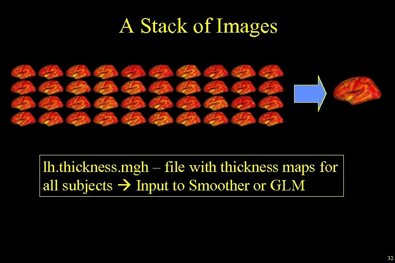
A Stack of Images lh. thickness. mgh – file with thickness maps for all subjects Input to Smoother or GLM 32
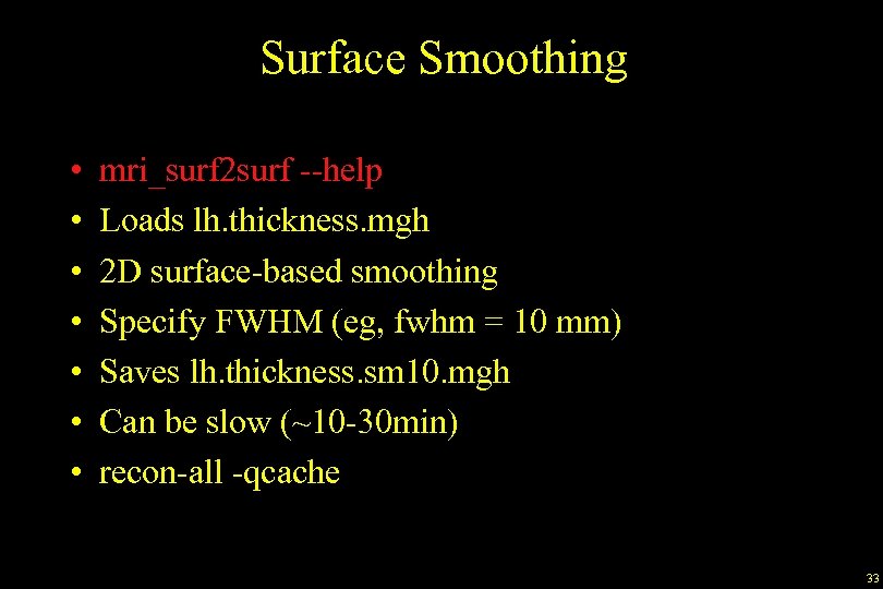
Surface Smoothing • • mri_surf 2 surf --help Loads lh. thickness. mgh 2 D surface-based smoothing Specify FWHM (eg, fwhm = 10 mm) Saves lh. thickness. sm 10. mgh Can be slow (~10 -30 min) recon-all -qcache 33
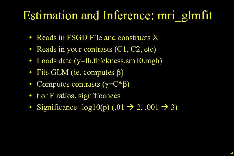
Estimation and Inference: mri_glmfit • • Reads in FSGD File and constructs X Reads in your contrasts (C 1, C 2, etc) Loads data (y=lh. thickness. sm 10. mgh) Fits GLM (ie, computes b) Computes contrasts (g=C*b) t or F ratios, significances Significance -log 10(p) (. 01 2, . 001 3) 34
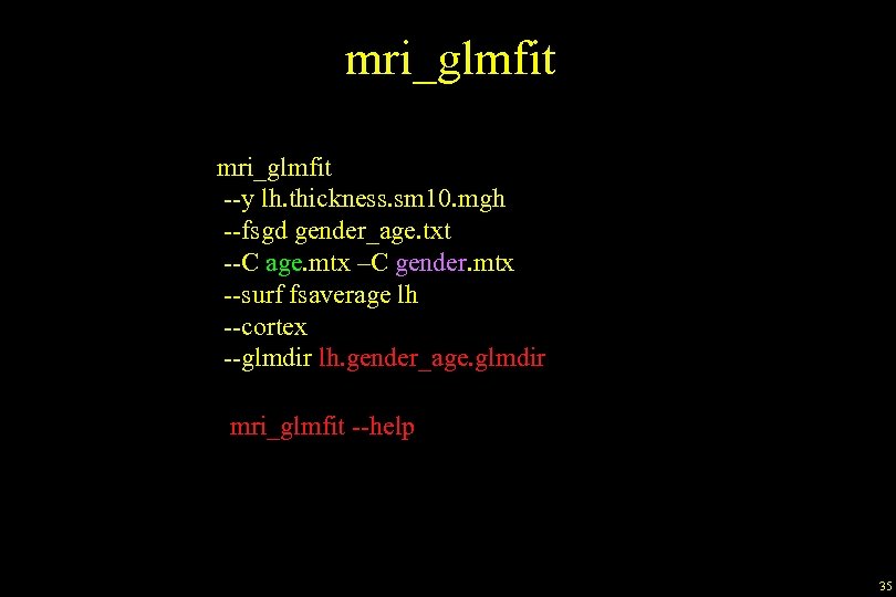
mri_glmfit --y lh. thickness. sm 10. mgh --fsgd gender_age. txt --C age. mtx –C gender. mtx --surf fsaverage lh --cortex --glmdir lh. gender_age. glmdir mri_glmfit --help 35
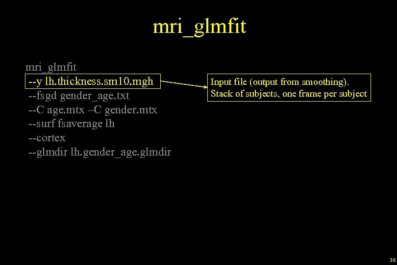
mri_glmfit --y lh. thickness. sm 10. mgh --fsgd gender_age. txt --C age. mtx –C gender. mtx --surf fsaverage lh --cortex --glmdir lh. gender_age. glmdir Input file (output from smoothing). Stack of subjects, one frame per subject 36
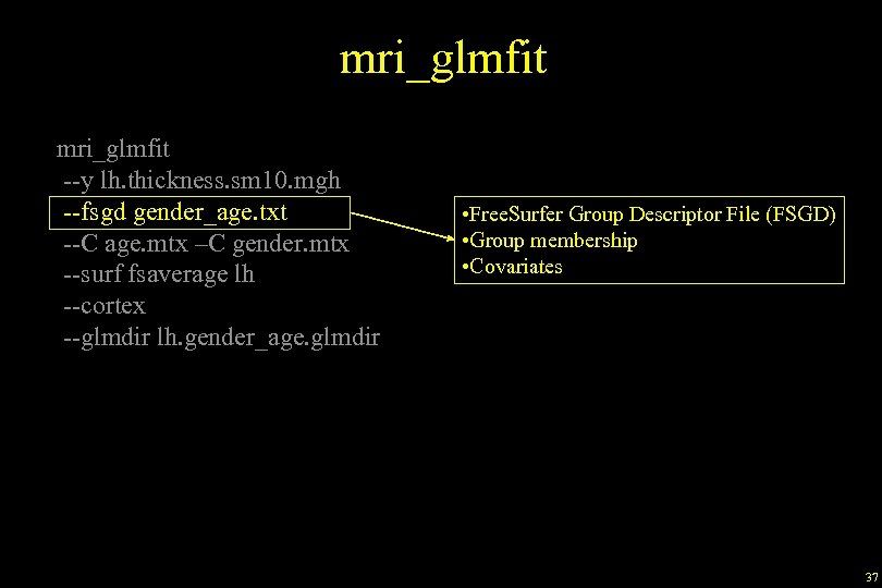
mri_glmfit --y lh. thickness. sm 10. mgh --fsgd gender_age. txt --C age. mtx –C gender. mtx --surf fsaverage lh --cortex --glmdir lh. gender_age. glmdir • Free. Surfer Group Descriptor File (FSGD) • Group membership • Covariates 37
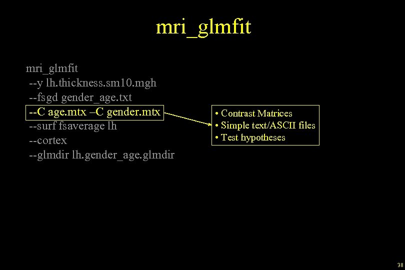
mri_glmfit --y lh. thickness. sm 10. mgh --fsgd gender_age. txt --C age. mtx –C gender. mtx --surf fsaverage lh --cortex --glmdir lh. gender_age. glmdir • Contrast Matrices • Simple text/ASCII files • Test hypotheses 38
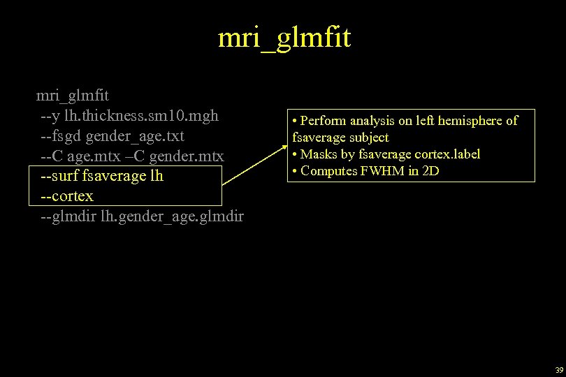
mri_glmfit --y lh. thickness. sm 10. mgh --fsgd gender_age. txt --C age. mtx –C gender. mtx --surf fsaverage lh --cortex --glmdir lh. gender_age. glmdir • Perform analysis on left hemisphere of fsaverage subject • Masks by fsaverage cortex. label • Computes FWHM in 2 D 39
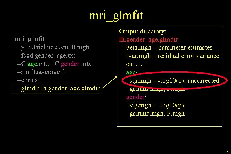
mri_glmfit --y lh. thickness. sm 10. mgh --fsgd gender_age. txt --C age. mtx –C gender. mtx --surf fsaverage lh --cortex --glmdir lh. gender_age. glmdir Output directory: lh. gender_age. glmdir/ beta. mgh – parameter estimates rvar. mgh – residual error variance etc … age/ sig. mgh = -log 10(p), uncorrected gamma. mgh, F. mgh gender/ sig. mgh = -log 10(p) gamma. mgh, F. mgh 40
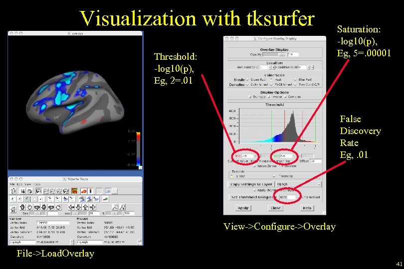
Visualization with tksurfer Threshold: -log 10(p), Eg, 2=. 01 Saturation: -log 10(p), Eg, 5=. 00001 False Discovery Rate Eg, . 01 View->Configure->Overlay File->Load. Overlay 41
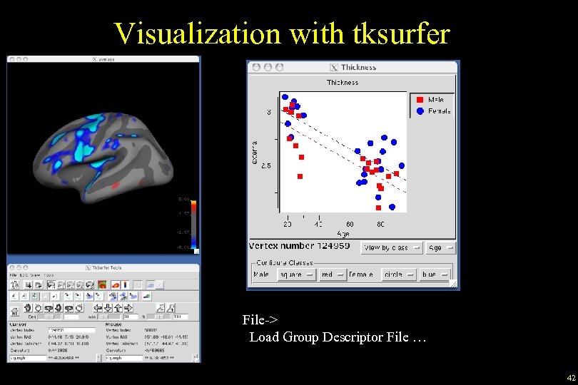
Visualization with tksurfer File-> Load Group Descriptor File … 42
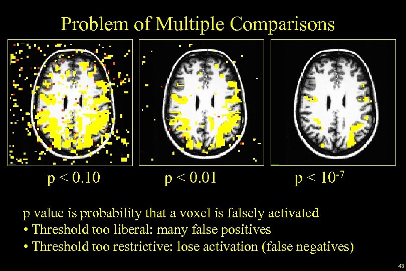
Problem of Multiple Comparisons p < 0. 10 p < 0. 01 p < 10 -7 p value is probability that a voxel is falsely activated • Threshold too liberal: many false positives • Threshold too restrictive: lose activation (false negatives) 43
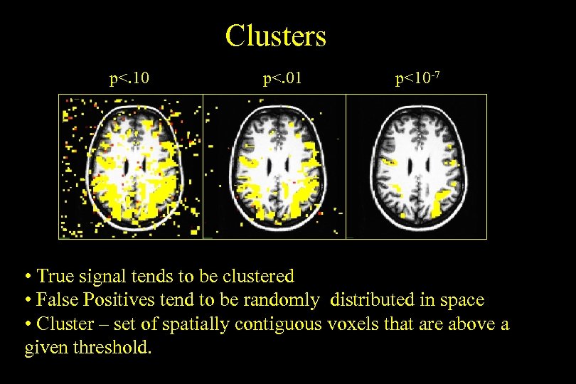
Clusters p<. 10 p<. 01 p<10 -7 • True signal tends to be clustered • False Positives tend to be randomly distributed in space • Cluster – set of spatially contiguous voxels that are above a given threshold.
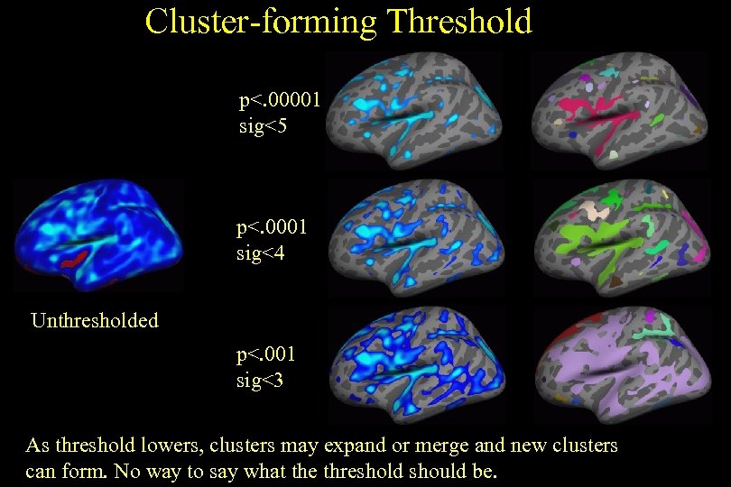
Cluster-forming Threshold p<. 00001 sig<5 p<. 0001 sig<4 Unthresholded p<. 001 sig<3 As threshold lowers, clusters may expand or merge and new clusters can form. No way to say what the threshold should be.
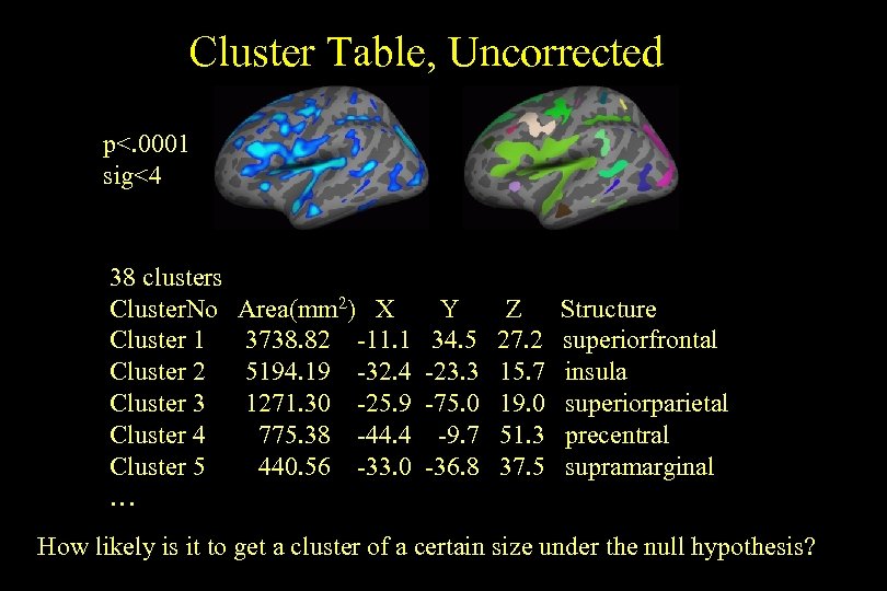
Cluster Table, Uncorrected p<. 0001 sig<4 38 clusters Cluster. No Cluster 1 Cluster 2 Cluster 3 Cluster 4 Cluster 5 … Area(mm 2) X 3738. 82 -11. 1 5194. 19 -32. 4 1271. 30 -25. 9 775. 38 -44. 4 440. 56 -33. 0 Y 34. 5 -23. 3 -75. 0 -9. 7 -36. 8 Z 27. 2 15. 7 19. 0 51. 3 37. 5 Structure superiorfrontal insula superiorparietal precentral supramarginal How likely is it to get a cluster of a certain size under the null hypothesis?
Correction for Multiple Comparisons • Cluster-based – Monte Carlo simulation – Permutation Tests • False Discovery Rate (FDR) – built into tksurfer and QDEC. (Genovese, et al, NI 2002) 47
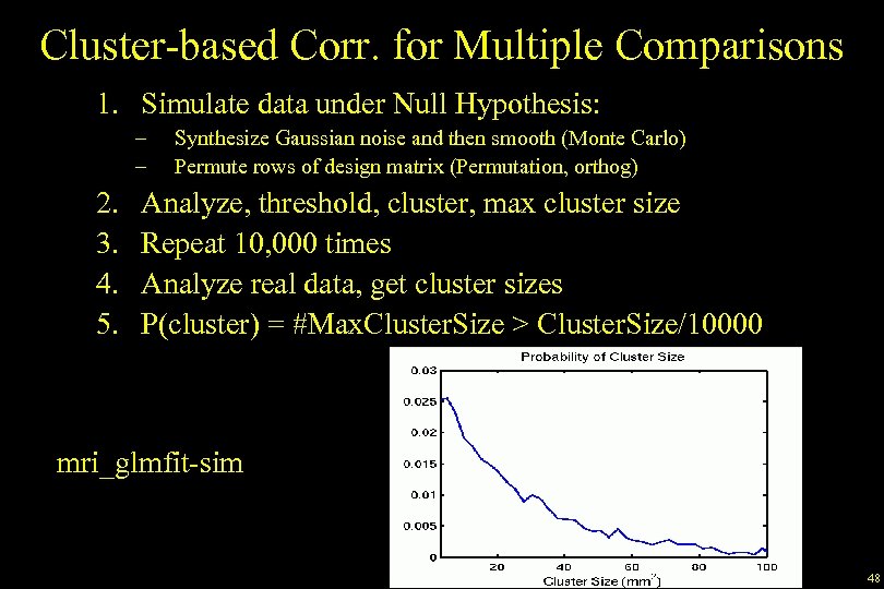
Cluster-based Corr. for Multiple Comparisons 1. Simulate data under Null Hypothesis: – – 2. 3. 4. 5. Synthesize Gaussian noise and then smooth (Monte Carlo) Permute rows of design matrix (Permutation, orthog) Analyze, threshold, cluster, max cluster size Repeat 10, 000 times Analyze real data, get cluster sizes P(cluster) = #Max. Cluster. Size > Cluster. Size/10000 mri_glmfit-sim 48
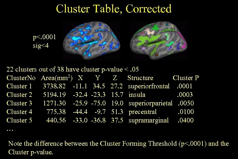
Cluster Table, Corrected p<. 0001 sig<4 22 clusters out of 38 have cluster p-value <. 05 Cluster. No Area(mm 2) X Y Z Structure Cluster P Cluster 1 3738. 82 -11. 1 34. 5 27. 2 superiorfrontal. 0001 Cluster 2 5194. 19 -32. 4 -23. 3 15. 7 insula. 0003 Cluster 3 1271. 30 -25. 9 -75. 0 19. 0 superiorparietal. 0050 Cluster 4 775. 38 -44. 4 -9. 7 51. 3 precentral. 0100 Cluster 5 440. 56 -33. 0 -36. 8 37. 5 supramarginal. 0400 … Note the difference between the Cluster Forming Threshold (p<. 0001) and the Cluster p-value.
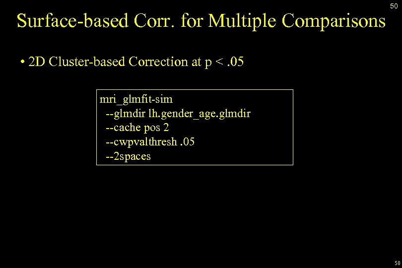
Surface-based Corr. for Multiple Comparisons 50 • 2 D Cluster-based Correction at p <. 05 mri_glmfit-sim --glmdir lh. gender_age. glmdir --cache pos 2 --cwpvalthresh. 05 --2 spaces 50
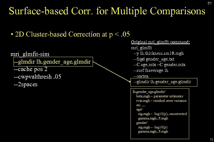
Surface-based Corr. for Multiple Comparisons 51 • 2 D Cluster-based Correction at p <. 05 mri_glmfit-sim --glmdir lh. gender_age. glmdir --cache pos 2 --cwpvalthresh. 05 --2 spaces Original mri_glmfit command: mri_glmfit --y lh. thickness. sm 10. mgh --fsgd gender_age. txt --C age. mtx –C gender. mtx --surf fsaverage lh --cortex --glmdir lh. gender_age. glmdir/ beta. mgh – parameter estimates rvar. mgh – residual error variance etc … age/ sig. mgh – -log 10(p), uncorrected gamma. mgh, F. mgh gender/ sig. mgh – -log 10(p) gamma. mgh, F. mgh 51
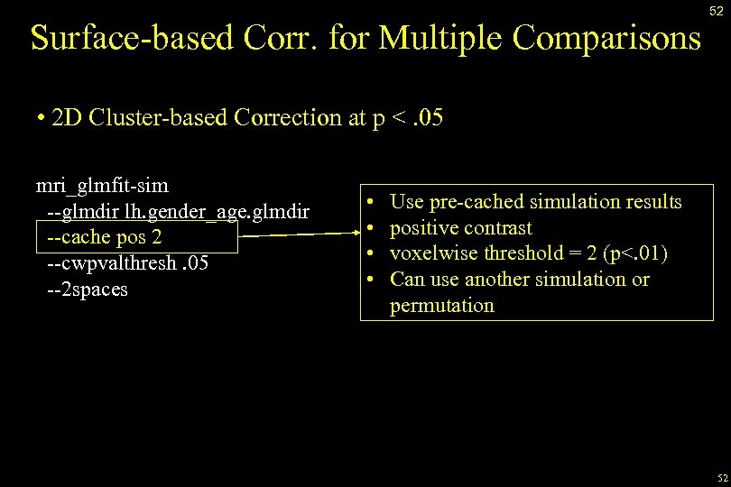
Surface-based Corr. for Multiple Comparisons 52 • 2 D Cluster-based Correction at p <. 05 mri_glmfit-sim --glmdir lh. gender_age. glmdir --cache pos 2 --cwpvalthresh. 05 --2 spaces • • Use pre-cached simulation results positive contrast voxelwise threshold = 2 (p<. 01) Can use another simulation or permutation 52
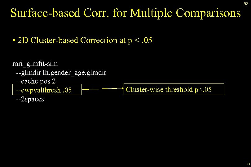
Surface-based Corr. for Multiple Comparisons 53 • 2 D Cluster-based Correction at p <. 05 mri_glmfit-sim --glmdir lh. gender_age. glmdir --cache pos 2 --cwpvalthresh. 05 --2 spaces Cluster-wise threshold p<. 05 53
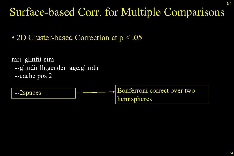
Surface-based Corr. for Multiple Comparisons 54 • 2 D Cluster-based Correction at p <. 05 mri_glmfit-sim --glmdir lh. gender_age. glmdir --cache pos 2 --cwpvalthresh. 05 --2 spaces Bonferroni correct over two hemispheres 54
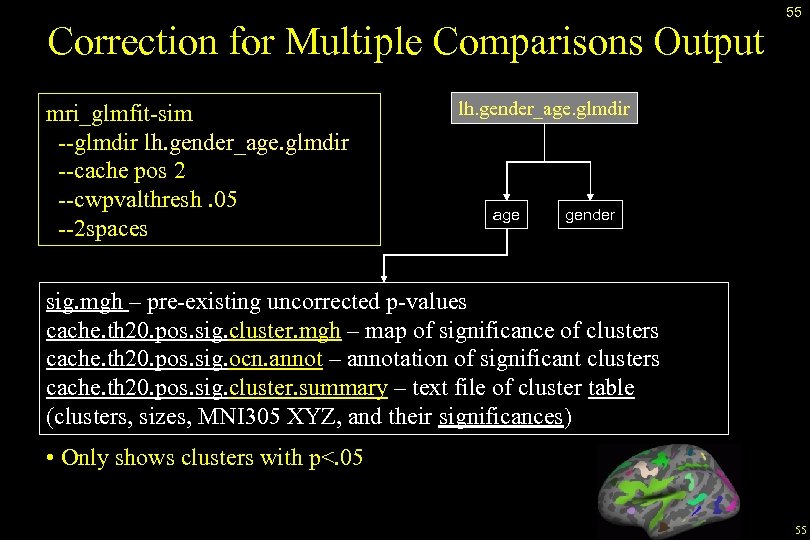
Correction for Multiple Comparisons Output mri_glmfit-sim --glmdir lh. gender_age. glmdir --cache pos 2 --cwpvalthresh. 05 --2 spaces 55 lh. gender_age. glmdir age gender sig. mgh – pre-existing uncorrected p-values cache. th 20. pos. sig. cluster. mgh – map of significance of clusters cache. th 20. pos. sig. ocn. annot – annotation of significant clusters cache. th 20. pos. sig. cluster. summary – text file of cluster table (clusters, sizes, MNI 305 XYZ, and their significances) • Only shows clusters with p<. 05 55
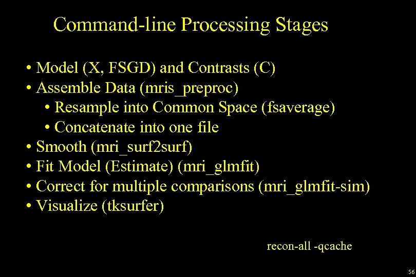
Command-line Processing Stages • Model (X, FSGD) and Contrasts (C) • Assemble Data (mris_preproc) • Resample into Common Space (fsaverage) • Concatenate into one file • Smooth (mri_surf 2 surf) • Fit Model (Estimate) (mri_glmfit) • Correct for multiple comparisons (mri_glmfit-sim) • Visualize (tksurfer) recon-all -qcache 56
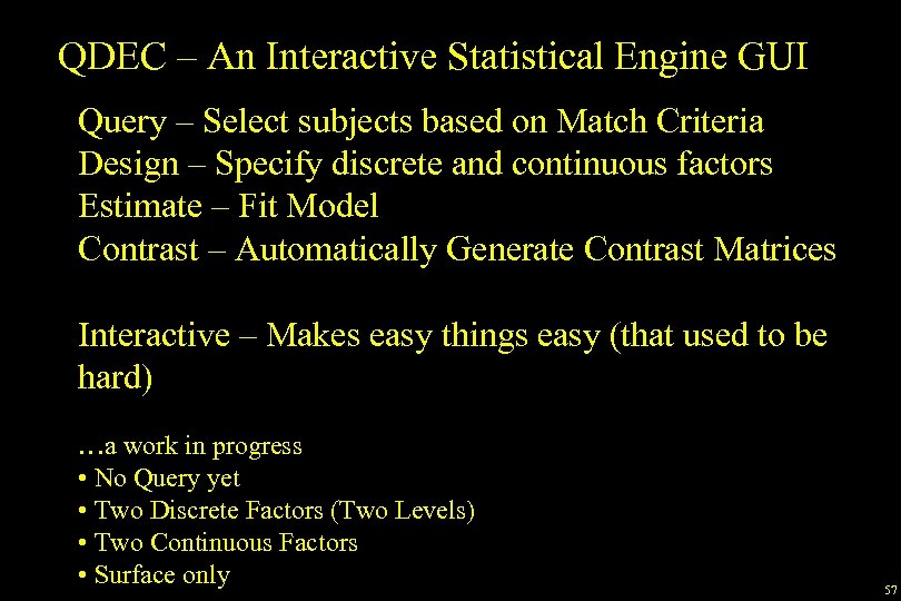
QDEC – An Interactive Statistical Engine GUI Query – Select subjects based on Match Criteria Design – Specify discrete and continuous factors Estimate – Fit Model Contrast – Automatically Generate Contrast Matrices Interactive – Makes easy things easy (that used to be hard) …a work in progress • No Query yet • Two Discrete Factors (Two Levels) • Two Continuous Factors • Surface only 57
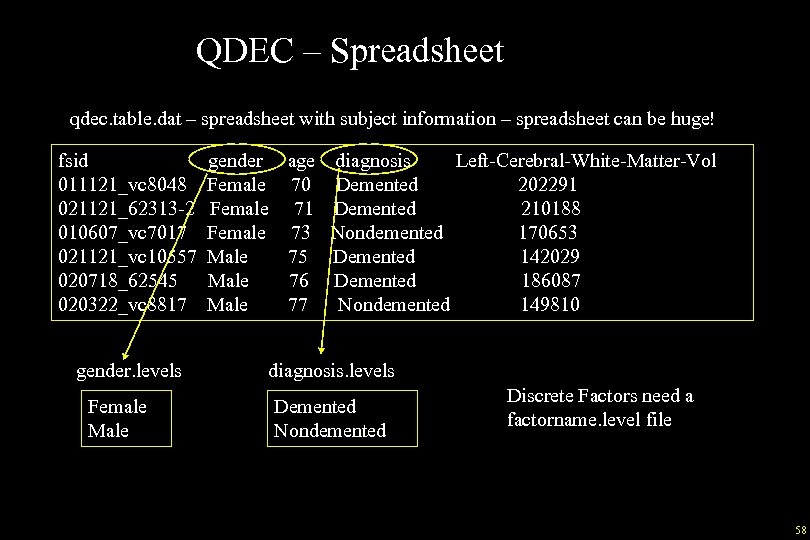
QDEC – Spreadsheet qdec. table. dat – spreadsheet with subject information – spreadsheet can be huge! fsid 011121_vc 8048 021121_62313 -2 010607_vc 7017 021121_vc 10557 020718_62545 020322_vc 8817 gender. levels Female Male gender age diagnosis Left-Cerebral-White-Matter-Vol Female 70 Demented 202291 Female 71 Demented 210188 Female 73 Nondemented 170653 Male 75 Demented 142029 Male 76 Demented 186087 Male 77 Nondemented 149810 diagnosis. levels Demented Nondemented Discrete Factors need a factorname. level file 58
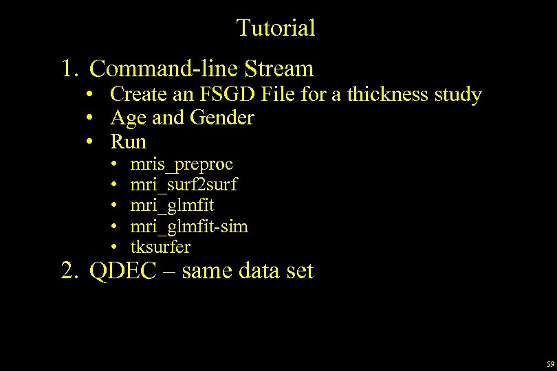
Tutorial 1. Command-line Stream • Create an FSGD File for a thickness study • Age and Gender • Run • • • mris_preproc mri_surf 2 surf mri_glmfit-sim tksurfer 2. QDEC – same data set 59
End of Presentation 60
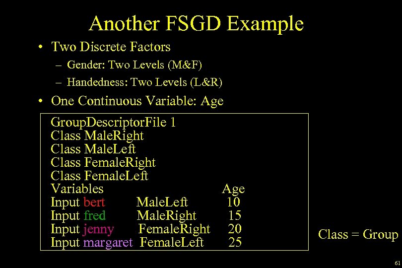
Another FSGD Example • Two Discrete Factors – Gender: Two Levels (M&F) – Handedness: Two Levels (L&R) • One Continuous Variable: Age Group. Descriptor. File 1 Class Male. Right Class Male. Left Class Female. Right Class Female. Left Variables Age Input bert Male. Left 10 Input fred Male. Right 15 Input jenny Female. Right 20 Input margaret Female. Left 25 Class = Group 61
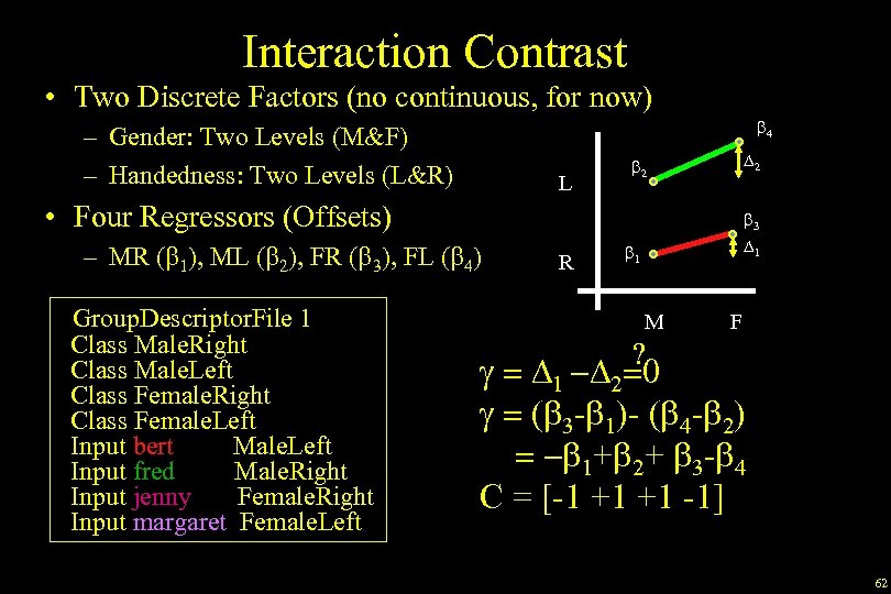
Interaction Contrast • Two Discrete Factors (no continuous, for now) b 4 – Gender: Two Levels (M&F) – Handedness: Two Levels (L&R) L D 2 b 2 • Four Regressors (Offsets) – MR (b 1), ML (b 2), FR (b 3), FL (b 4) Group. Descriptor. File 1 Class Male. Right Class Male. Left Class Female. Right Class Female. Left Input bert Male. Left Input fred Male. Right Input jenny Female. Right Input margaret Female. Left R b 3 D 1 b 1 M ? F g = D 1 -D 2=0 g = (b 3 -b 1)- (b 4 -b 2) = -b 1+b 2+ b 3 -b 4 C = [-1 +1 +1 -1] 62
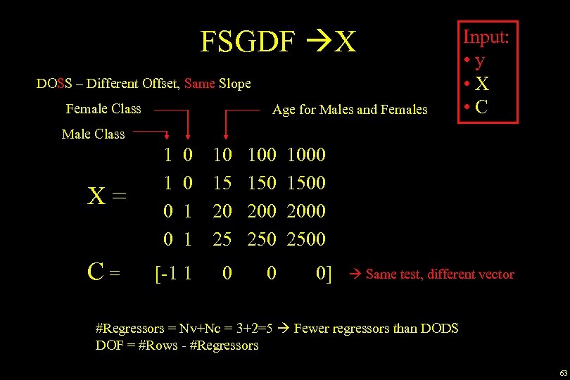
FSGDF X DOSS – Different Offset, Same Slope Female Class Age for Males and Females Input: • y • X • C Male Class X= 1 1 0 0 1 1 10 15 20 25 100 150 200 250 C= [-1 1 0 0 1000 1500 2000 2500 0] Same test, different vector #Regressors = Nv+Nc = 3+2=5 Fewer regressors than DODS DOF = #Rows - #Regressors 63
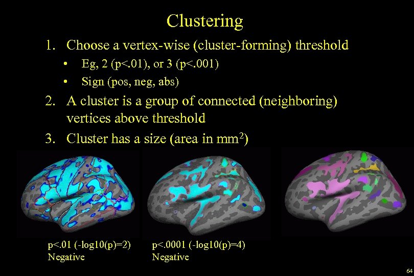
Clustering 1. Choose a vertex-wise (cluster-forming) threshold • • Eg, 2 (p<. 01), or 3 (p<. 001) Sign (pos, neg, abs) 2. A cluster is a group of connected (neighboring) vertices above threshold 3. Cluster has a size (area in mm 2) p<. 01 (-log 10(p)=2) Negative p<. 0001 (-log 10(p)=4) Negative 64
Surface Registration Subject 1 Subject 2 (Before) Subject 2 (After) • Shift, Rotate, Stretch • High dimensional (~500 k) • Preserve metric properties • Take variance into account 65 65
589c9e635a247de5d55b261af12b073a.ppt