Supply and Demand Chapter 2 1 introduction

Supply and Demand Chapter 2 1

introduction • why did the price of gasoline rise (around %16. 33) after hurricane Katrina (new orleans: August 2005)and hurricane rita (Texas: September 2005), although price of crude oil did not change significantly? • By early October 2005, %30 of U. S. refining capacity was shut down by the 2 storms. • by how much would the price (P) have fallen if 1/2 of the capacity came back? • to answer such questions, we use a model of supply and demand. 2

demand • a product’s demand curve (D) shows how much buyers of the product want to buy (QD)at each possible price (P), holding all other factors that affect demand constant. • Demand curve slopes downward to reflect the negative relationship between (P) and (Qd) • Factors affecting demand (population growth, tastes, income, prices of other goods, government regulations. 3

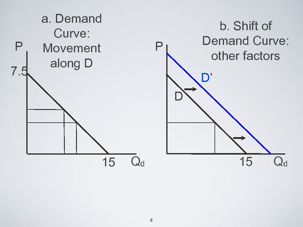P 7. 5 a. Demand Curve: Movement along D b. Shift of Demand Curve: other factors P D’ D 15 Qd 15 4 Qd

• Make sure to know the following: 1. substitutes and complements 2. inferior and Normal goods 2. Movements Along vs. Shifts of the demand curve. • Assignment 1 5

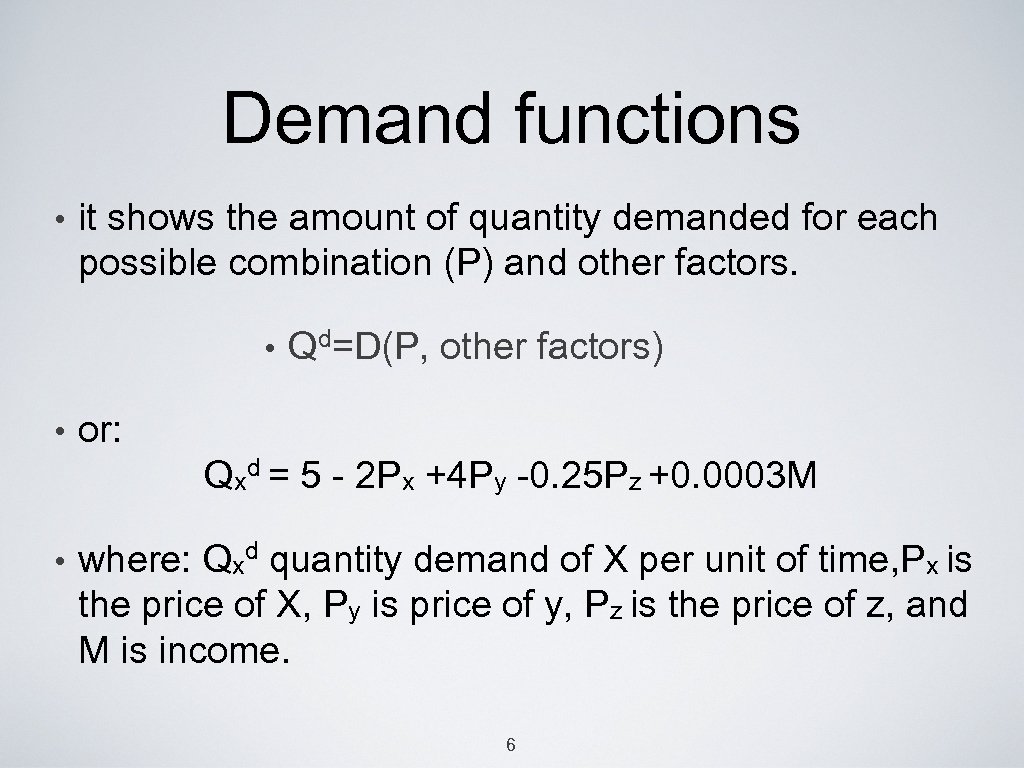Demand functions • it shows the amount of quantity demanded for each possible combination (P) and other factors. • • Qd=D(P, other factors) or: Qxd = 5 - 2 Px +4 Py -0. 25 Pz +0. 0003 M • where: Qxd quantity demand of X per unit of time, Px is the price of X, Py is price of y, Pz is the price of z, and M is income. 6

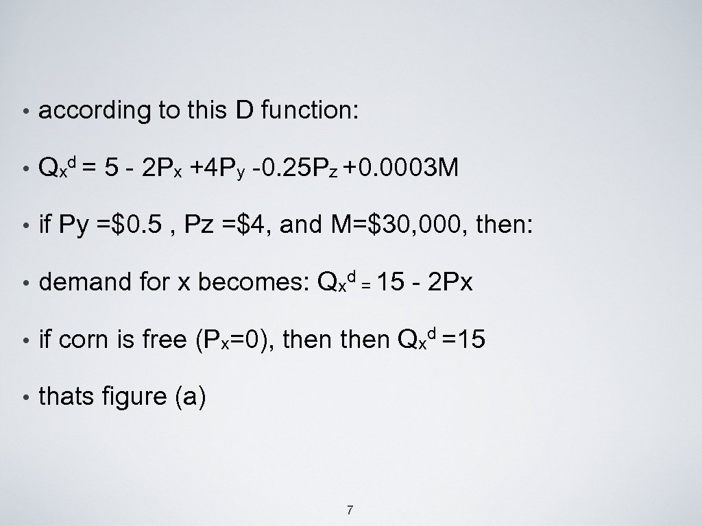• according to this D function: • Qxd = 5 - 2 Px +4 Py -0. 25 Pz +0. 0003 M • if Py =$0. 5 , Pz =$4, and M=$30, 000, then: • demand for x becomes: Qxd = 15 - 2 Px • if corn is free (Px=0), then Qxd =15 • thats figure (a) 7

• figure (b) shows shift in demand due to one of the factors affecting demand (not Px) • if Py is $0. 5 then QDX = 9 while it is 11 when Py = $1. 8

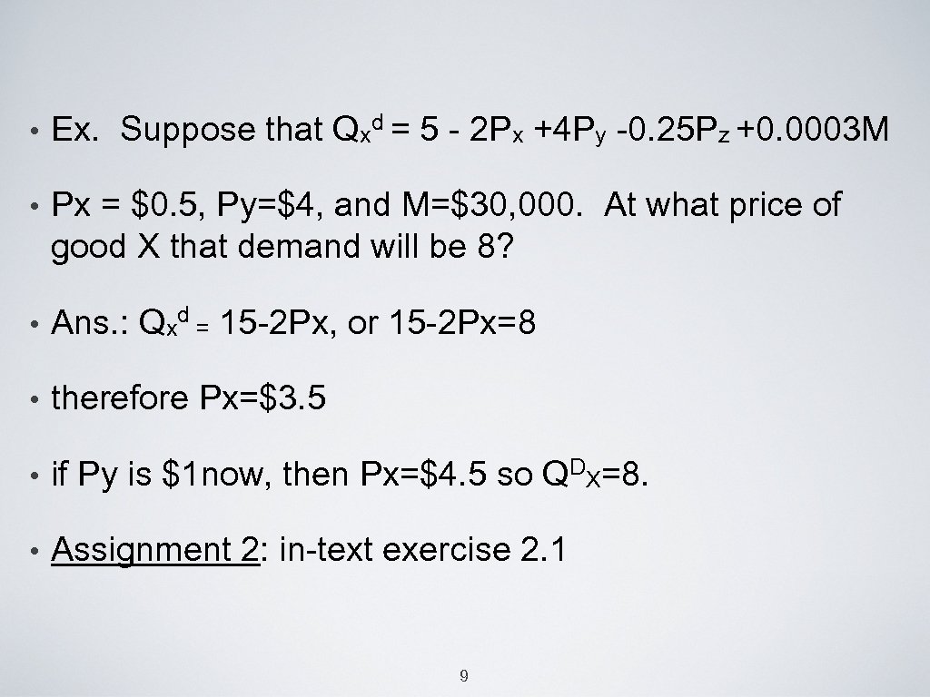• Ex. Suppose that Qxd = 5 - 2 Px +4 Py -0. 25 Pz +0. 0003 M • Px = $0. 5, Py=$4, and M=$30, 000. At what price of good X that demand will be 8? • Ans. : Qxd = 15 -2 Px, or 15 -2 Px=8 • therefore Px=$3. 5 • if Py is $1 now, then Px=$4. 5 so QDX=8. • Assignment 2: in-text exercise 2. 1 9

supply • this is the 2 nd part of the market • S curve shows how much sellers of a product want to sell at each possible price, holding fixed all other factors (determining S). 10

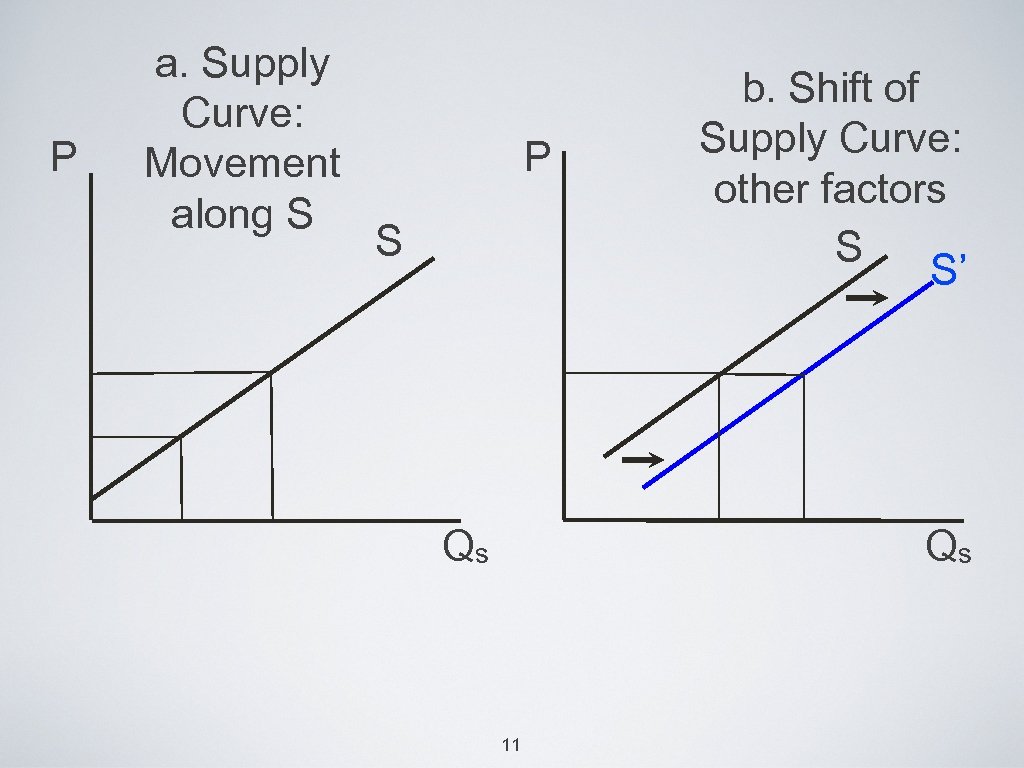P a. Supply Curve: Movement along S P S Qs b. Shift of Supply Curve: other factors S S’ Qs 11

• if P=3, then Qs=9 • if P=2, the Qs=4 • positive relationship between P and Qs • when P is higher, producing and selling the product is more profitable. • Other factors: technology, input cost, price of other outputs, taxes and subsidies 12

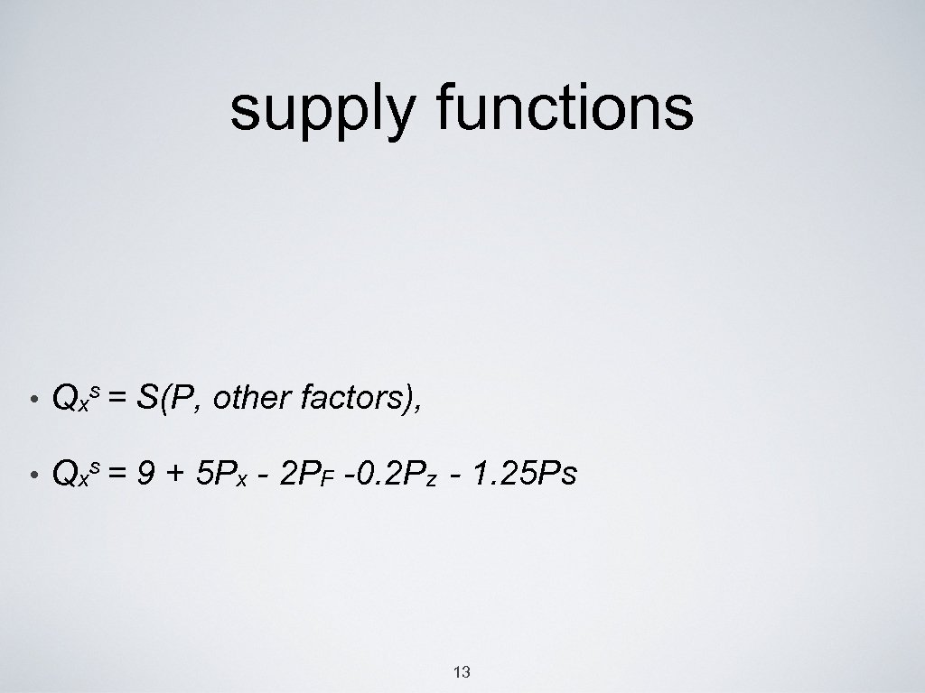supply functions • Qxs = S(P, other factors), • Qxs = 9 + 5 Px - 2 PF -0. 2 Pz - 1. 25 Ps 13

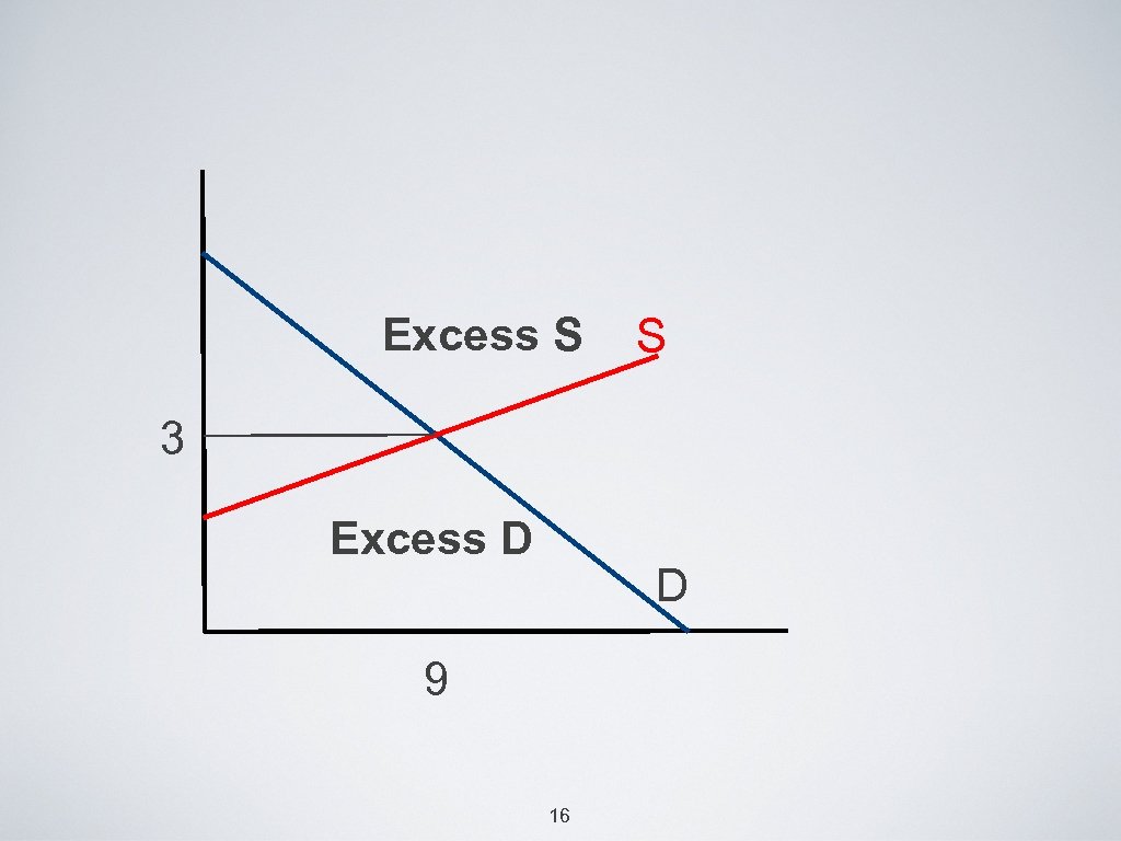
Market Equilibrium • after knowing D and S for a product, next step is to determine equilibrium P and Q. s=Qd Q • Thats when • The market clears at Pe. • Market prices tend to adjust so that Qs=Qd 14

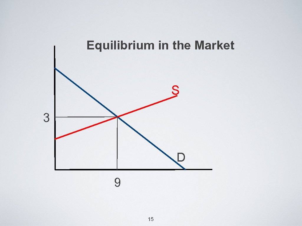Equilibrium in the Market S 3 D 9 15

Excess S S 3 Excess D D 9 16

• ex. : Qd=15 -2 P and Qs=5 P-6, what is the equilibrium price? • Qs=Qd • P=3 and QE=9 • Assignment III: in-text exercise 2. 2 17

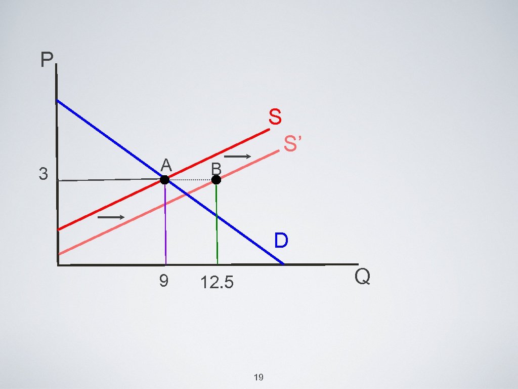
Changes in market equilibrium • if Pf fall from $2. 5 to $2, and Pz fall from $8 to $6, the supply curve will shift outward • after the shift, the market is not in equilibrium (at p=$3). • there is excess of. . ? 18

P S 3 A S’ B D 9 Q 12. 5 19

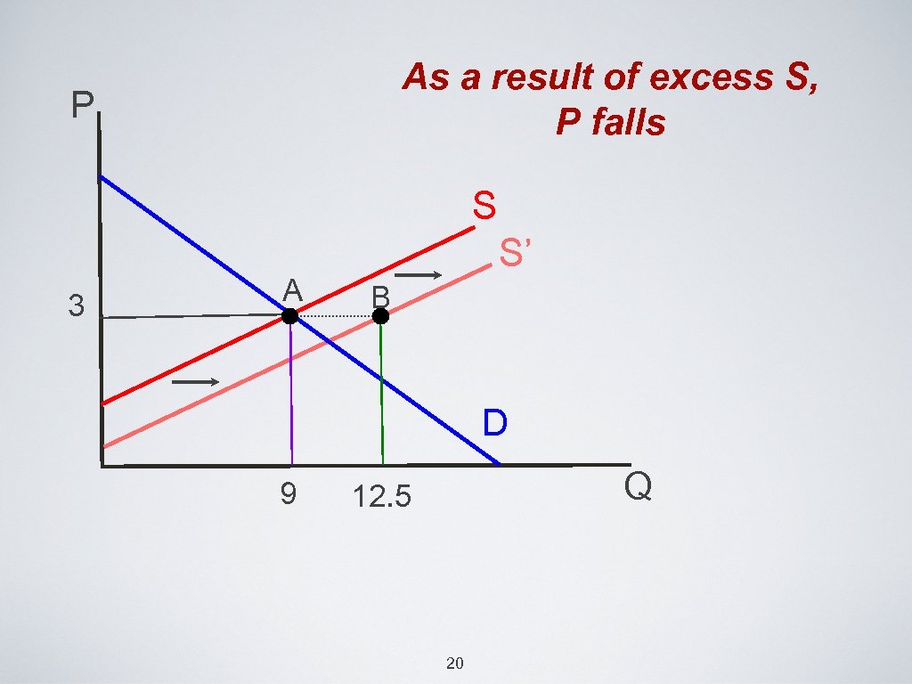As a result of excess S, P falls P S 3 A S’ B D 9 Q 12. 5 20

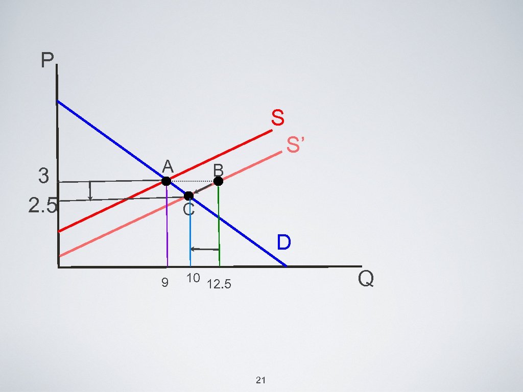P S 3 2. 5 S’ A B C D 9 Q 10 12. 5 21

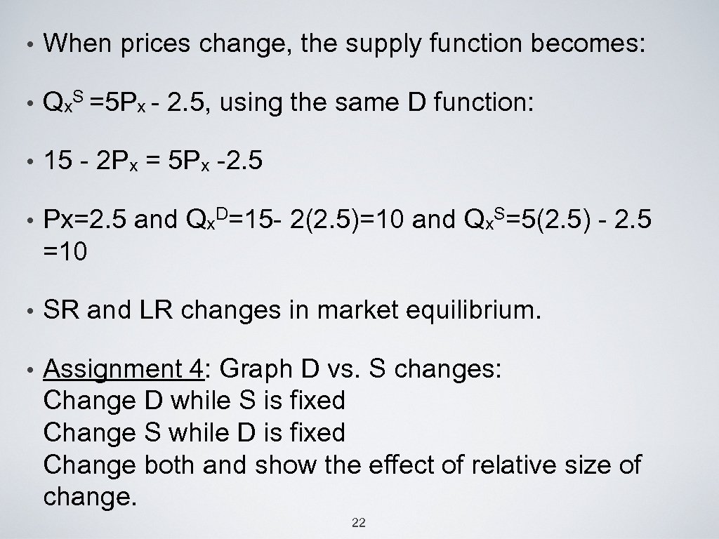• When prices change, the supply function becomes: • Qx. S =5 Px - 2. 5, using the same D function: • 15 - 2 Px = 5 Px -2. 5 • Px=2. 5 and Qx. D=15 - 2(2. 5)=10 and Qx. S=5(2. 5) - 2. 5 =10 • SR and LR changes in market equilibrium. • Assignment 4: Graph D vs. S changes: Change D while S is fixed Change S while D is fixed Change both and show the effect of relative size of change. 22

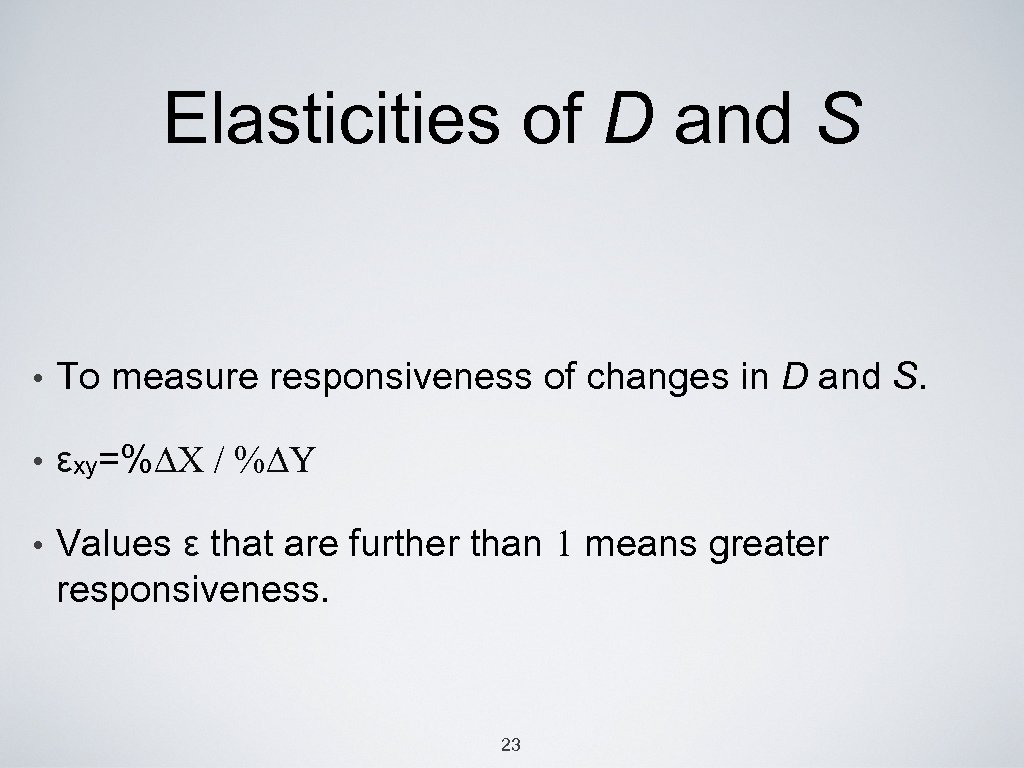Elasticities of D and S • To measure responsiveness of changes in D and S. • εxy=%∆X • / %∆Y Values ε that are further than 1 means greater responsiveness. 23

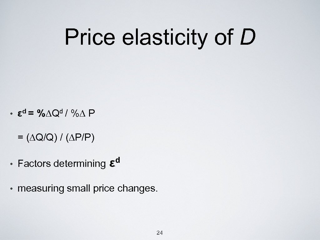Price elasticity of D • εd = %∆Qd / %∆ P = (∆Q/Q) / (∆P/P) • Factors determining εd • measuring small price changes. 24

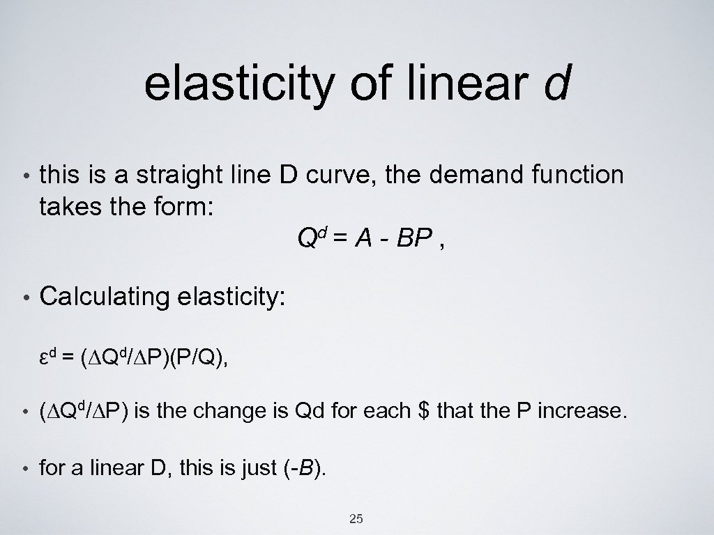elasticity of linear d • this is a straight line D curve, the demand function takes the form: Qd = A - BP , • Calculating elasticity: εd = (∆Qd/∆P)(P/Q), • (∆Qd/∆P) is the change is Qd for each $ that the P increase. • for a linear D, this is just (-B). 25

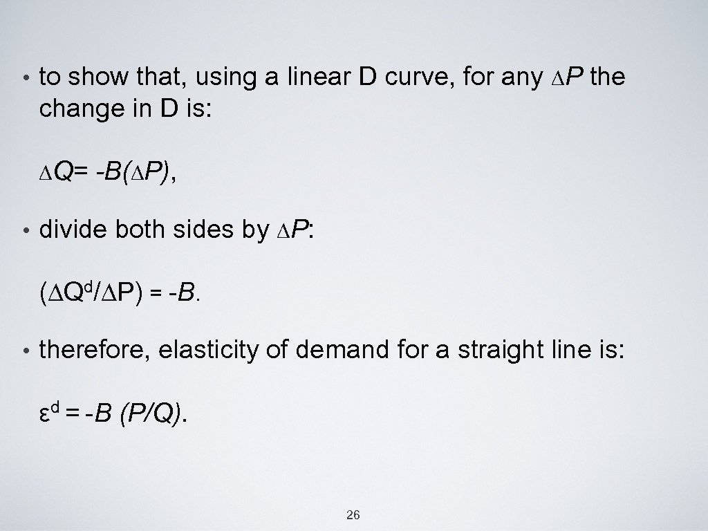• to show that, using a linear D curve, for any ∆P the change in D is: ∆Q= -B(∆P), • divide both sides by ∆P: (∆Qd/∆P) = -B. • therefore, elasticity of demand for a straight line is: εd = -B (P/Q). 26

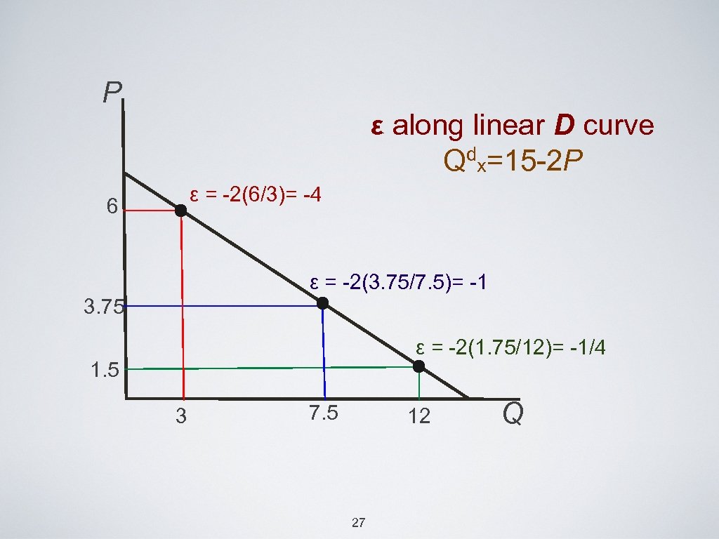P ε along linear D curve Qdx=15 -2 P ε = -2(6/3)= -4 6 ε = -2(3. 75/7. 5)= -1 3. 75 ε = -2(1. 75/12)= -1/4 1. 5 3 7. 5 12 27 Q

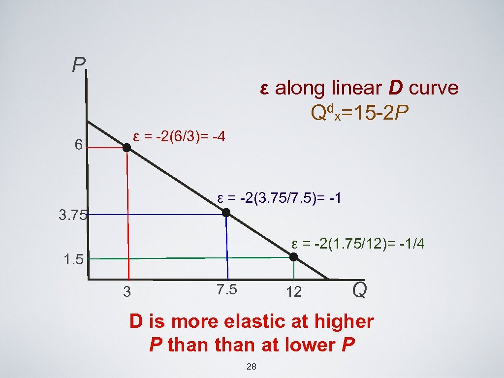P ε along linear D curve Qdx=15 -2 P ε = -2(6/3)= -4 6 ε = -2(3. 75/7. 5)= -1 3. 75 ε = -2(1. 75/12)= -1/4 1. 5 3 7. 5 12 Q D is more elastic at higher P than at lower P 28

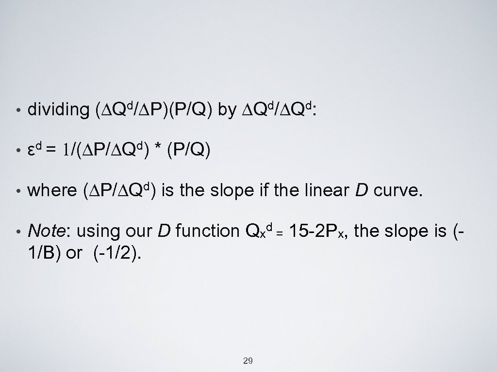• dividing (∆Qd/∆P)(P/Q) by ∆Qd/∆Qd: • εd = 1/(∆P/∆Qd) * (P/Q) • where (∆P/∆Qd) is the slope if the linear D curve. • Note: using our D function Qxd = 15 -2 Px, the slope is (1/B) or (-1/2). 29

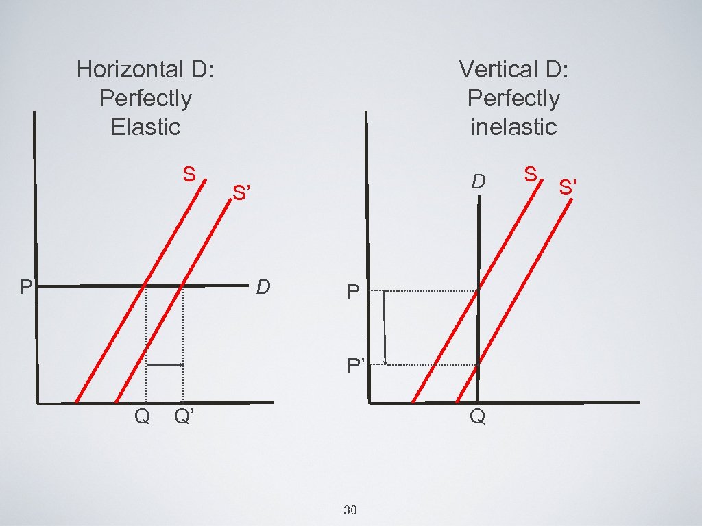Horizontal D: Perfectly Elastic S P Vertical D: Perfectly inelastic D S’ D P P’ Q Q’ Q 30 S S’

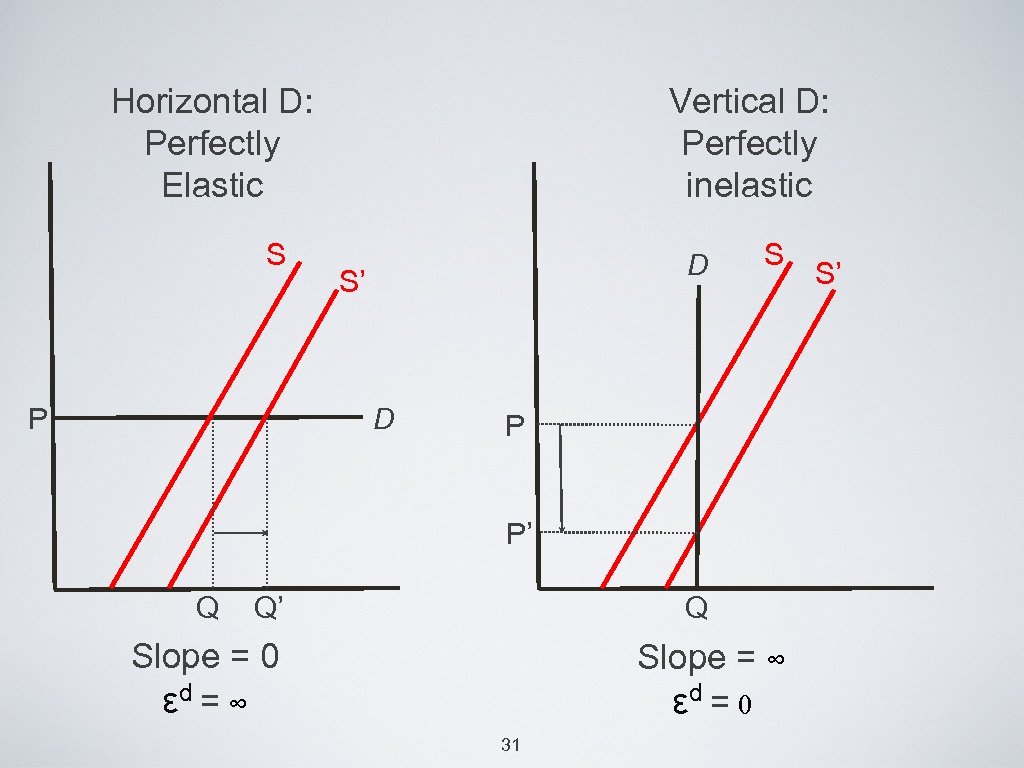Horizontal D: Perfectly Elastic S P Vertical D: Perfectly inelastic D S’ D S P P’ Q Q’ Q Slope = 0 εd = ∞ Slope = ∞ εd = 0 31 S’

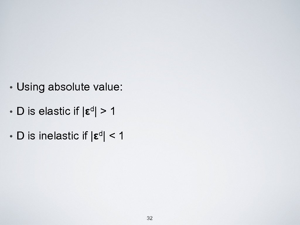• Using absolute value: d| |ε • D is elastic if >1 • D is inelastic if |εd| < 1 32

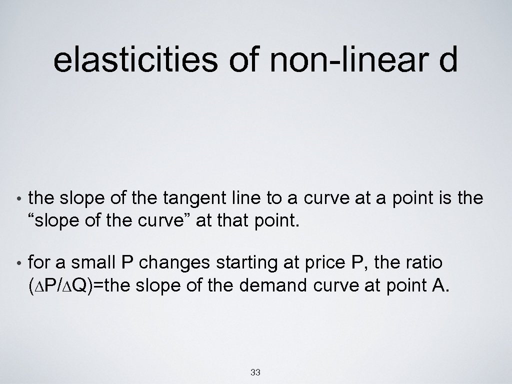elasticities of non-linear d • the slope of the tangent line to a curve at a point is the “slope of the curve” at that point. • for a small P changes starting at price P, the ratio (∆P/∆Q)=the slope of the demand curve at point A. 33

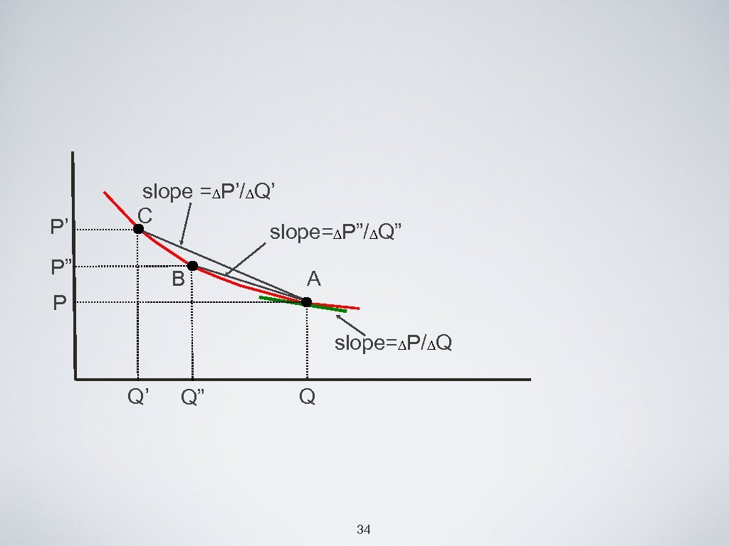P’ slope =∆P’/∆Q’ C slope=∆P”/∆Q” P” B A P slope=∆P/∆Q Q’ Q” Q 34

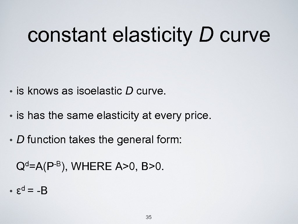constant elasticity D curve • is knows as isoelastic D curve. • is has the same elasticity at every price. • D function takes the general form: Qd=A(P-B), WHERE A>0, B>0. • εd = -B 35

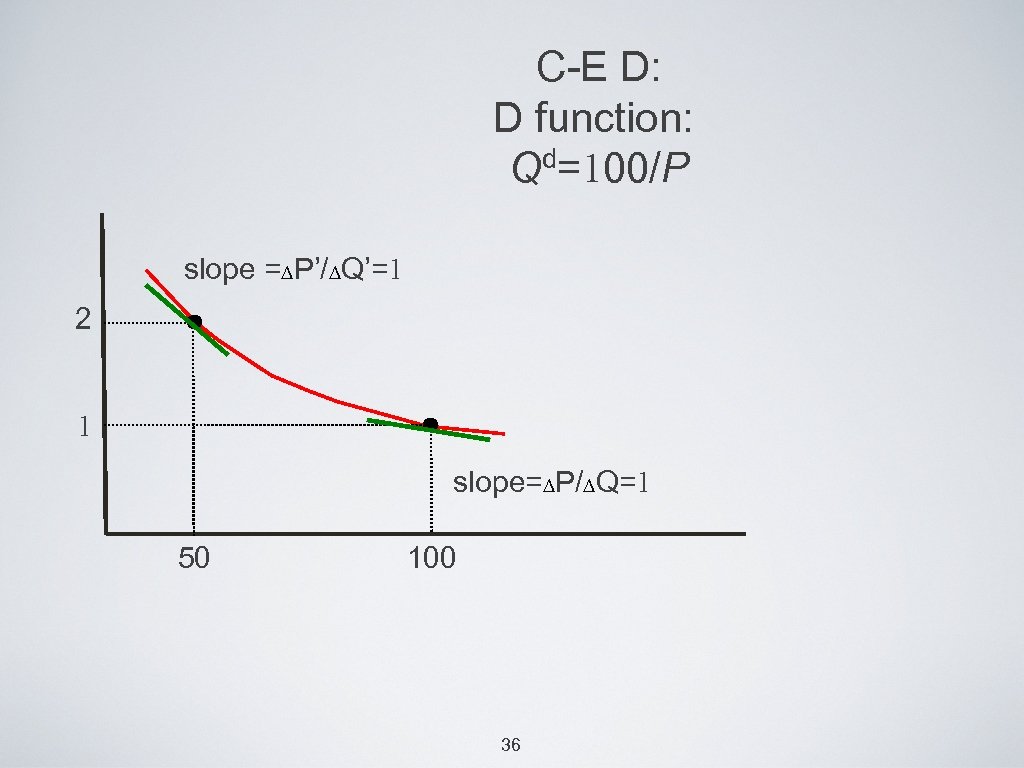C-E D: D function: Qd=100/P slope =∆P’/∆Q’=1 2 1 slope=∆P/∆Q=1 50 100 36

total Expenditure and elasticity of D • elasticity of D shows how TE changes when P increases and we move along the D curve. • TE=PQ • TE will increase for a small P increase when D is inelastic and decrease when D is elastic. • Since Total revenue (TR) always =TE, the same is true for sellers’ revenue. (TR and εd) 37

price elasticity of s • εd = (1/(∆P/∆Q))*(P/Q), where (∆P/∆Q) is the slope of S curve. • Perfectly elastic S. • Perfectly inelastic supply. 38

other elasticities • income elasticity of demand • cross-price elasticity of demand 39