Summary of First Section Deterministic Analysis John H

Summary of First Section: Deterministic Analysis John H. Vande Vate Spring, 2007 1 1

Where We’ve Been • Introduction to modes and transportation rates – There are economies of scale in transportation costs – Consolidation helps us capitalize on these economies of scale 2 2

Where We’ve Been • Introduction to Finance & SCM – Economic Profit – Focus on Working Capital • Days of Inventory • Days Sales Outstanding • Days Purchases Outstanding – Cost of Holding Inventory • Capital charge • Non-capital charge 3 3

Where We’ve Been • Transportation & “Deterministic” Inventory – Pipeline Inventory – Cycle Inventory – Simple Example to illustrate • How to estimate, transportation & inventory costs • The “magic” of consolidation • The EOQ: Balancing Transport & Inventory costs • Network Models – Quick review of network flows – Adding reality • Weight & Cube • Concave costs • Some aspects of Time 4 4

Where We’ve Been • Consolidation – Consolidating LTL shipments • Costs • Basic model • Integrality? : Should assignments of customers to consolidation points be binary? • Integrality? – In Favor: Simplicity. – Against: Reality 5 5

Reality • Our assumption: – Annual demand is evenly spread across the year (No seasonality, No variability) • The Reality: – Individual customer demands vary widely from day -to-day, week-to-week, month-to-month • The Impact: – We plan to run full trucks – In reality sometimes they are not full, other times there’s more than they can carry. • Our model ignores this – we do incorporate a load (fudge) factor 6 6

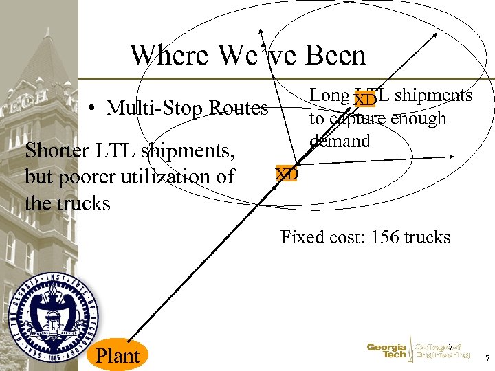Where We’ve Been Long XD shipments LTL to capture enough demand • Multi-Stop Routes Shorter LTL shipments, but poorer utilization of the trucks XD Fixed cost: 156 trucks Plant 7 7

Where We’ve Been • Multi-Stop Routes – Use Column Generation to find a small set of good multi-stop routes – Two Complications • A Route entails several variables – Route. Volume: how much volume we carry on this route for a given consolidation point – Multi. Stop. Trucks: how many trucks we run on this route What columns do we generate? • The constraints in the Master problem that relate Multi. Stop. Trucks to Route. Volumes Normally in Column Generation we don’t add constraints as we add columns. – Case 1: Constraint is not relevant – Case 2: Constraint is tight 8 8

Where We’ve Been • Load-Driven Consolidation – When we are concerned about cost of transportation first, then level of service – Low value, thin margins, high volume • Consolidate to improve service • Full truck load to each store is – Impractical (small format stores) – Creates too much (cycle) inventory – Forces us to forecast demand at the store level far in advance 9 9

Where We’ve Been • Objective is transport costs – Line haul to pools – Delivery from pools to stores • Service as a constraint • Trailer Fill: Max Time to Fill Trailer • Example: OTD < 6 days – – Order processing: 1 day Batching & Picking: 1 day Line Haul: 3 days 2 days Trailer Fill 1 day 2 days 10 10

Where We’re Going • Location: – We assumed the choices for potential consolidation were given – How do we identify good choices? • Stochastic Analysis – Introduction to Stochastic Variability – Retail Pricing: Markdowns as a % of Sales have risen steadily to over 30% – Sport Obermeyer • The relationship between forecasting, sourcing, and markdowns – Managing Inventory: Replenishment – Postponement & Push vs Pull • Applications – BMW and the Bullwhip Effect – Your projects 11 11

The Exam • • • Laptops not permitted 4 -5 questions Did you understand? Can you interpret for the business? Some modeling 12 12

Models • Define your variables and parameters clearly, give units. Use clear mnemonics • Brief description of what each constraint accomplishes • Clear and unambiguous indexing • Pseudo AMPL is fine • Expect to need to read (but not produce) AMPL models 13 13