Successes and Challenges for Flow Control Simulations Invited

Successes and Challenges for Flow Control Simulations (Invited) Christopher L. Rumsey NASA Langley Research Center Hampton, VA AIAA 2008 -4311 4 th AIAA Flow Control Conference, Seattle, WA 1

Outline • Introduction • Perspectives on 3 workshop cases – Synthetic Jet into Quiescent Air – Synthetic Jet in a Crossflow – Flow over a Hump Model • For each, summary given and remaining challenges identified 2

Introduction • Synthetic jets have many practical applications – Jet vectoring, separation control, enhanced mixing, skin friction reduction, virtual aeroshaping • How accurate is CFD for predicting these types of unsteady flows? • CFDVAL 2004 workshop was held in March 2004 and addressed this question – (http: //cfdval 2004. larc. nasa. gov) – Special issue of AIAA Journal (Vol 44, No 2, 2006) had summary paper and 6 CFD papers – Many other papers have appeared as well (both AIAA conference papers as well as in journals) • Purpose of this paper: Summarize progress and answer the questions – Has CFD gotten better at computing these types of flows? – Are more advanced methodologies being applied? – What challenges remain? 3

Introduction, cont’d • CFDVAL 2004 workshop – Case 1: Synthetic jet into quiescent air – Case 2: Synthetic jet in a crossflow – Case 3: Flow over a Hump model • Three conditions: no-flow-control, steady suction, oscillatory control • In ERCOFTAC database (Classic Collection), Case C. 83 • Overall summary from AIAA Journal, Vol 44 No 2, 2006 – CFD only able to qualitatively predict synthetic jet flow physics – In part due to uncertainty in how to model the BCs – Need identified: building-block experiments to focus on obtaining extremely detailed data at and near slot/orifice exits • A plug for workshops of this type: – – Many people computing same problems Improves synergy between CFDers and experimentalists Easier to discern trends & deficiencies “Outliers” easier to recognize 4

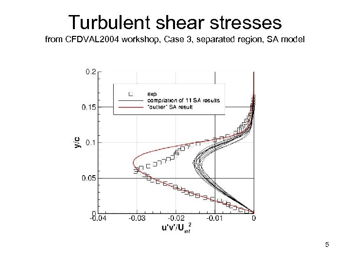Turbulent shear stresses from CFDVAL 2004 workshop, Case 3, separated region, SA model 5

Description of methodologies • Reduced-order or low-order – Simplifications to RANS/URANS – E. g. , lumped element models, quasi-one-D models, proper orthogonal decomposition (POD) models – Less expensive than RANS/URANS – Useful to find viable design from among hundreds of possibilities 6

Description of methodologies • RANS/URANS – Both solve Reynolds-averaged equations (RANS is steady-state, URANS is time-accurate) (incompressible) - Then equations written in terms of or phase-average) (long-time-average - End up with unclosed term(s), turbulent stress: - Modeled with turbulence model (e. g. , 1 -eqn, 2 -eqn, EASM, RSM): models the MEAN EFFECTS of turbulent fluctuations - RANS/URANS assumed to be valid if time scale of turbulent fluctuations << physical time step << important global unsteady time scales in the flow 7

Description of methodologies • LES & blended RANS/LES – Derived by applying low-pass filter to N-S eqns – Idea is to resolve larger turbulent eddies, model smaller ones – Resulting filtered eqns are functionally identical to RANS equations: again unclosed terms must be modeled – LES subgrid-scale (SGS) models are different from RANS turbulence models in that they include filter (typically dependent on local grid size) – Blended RANS/LES works by blending the SGS model and turbulence model • Sometimes problems in blending region (e. g. , if in log-layer) 8

Description of methodologies • LES & blended RANS/LES, cont’d – LES is difficult to analyze - easily complicated by numerics – Excessive numerical dissipation affects ability to resolve features – Numerical dissipation can behave like SGS model – This fact taken advantage of in implicit LES (ILES) • No SGS model used • Inherent numerical dissipation provides filtering needed at smallest scales • Theoretically justified in MILES (specific numerical methods employed) 9

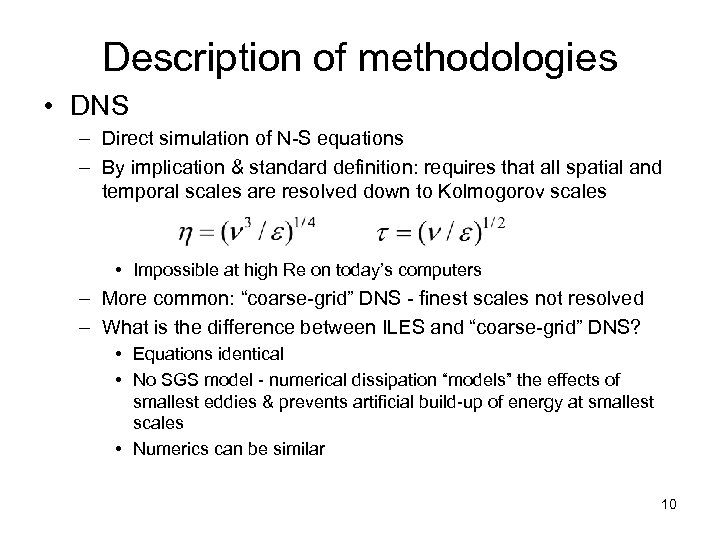Description of methodologies • DNS – Direct simulation of N-S equations – By implication & standard definition: requires that all spatial and temporal scales are resolved down to Kolmogorov scales • Impossible at high Re on today’s computers – More common: “coarse-grid” DNS - finest scales not resolved – What is the difference between ILES and “coarse-grid” DNS? • Equations identical • No SGS model - numerical dissipation “models” the effects of smallest eddies & prevents artificial build-up of energy at smallest scales • Numerics can be similar 10

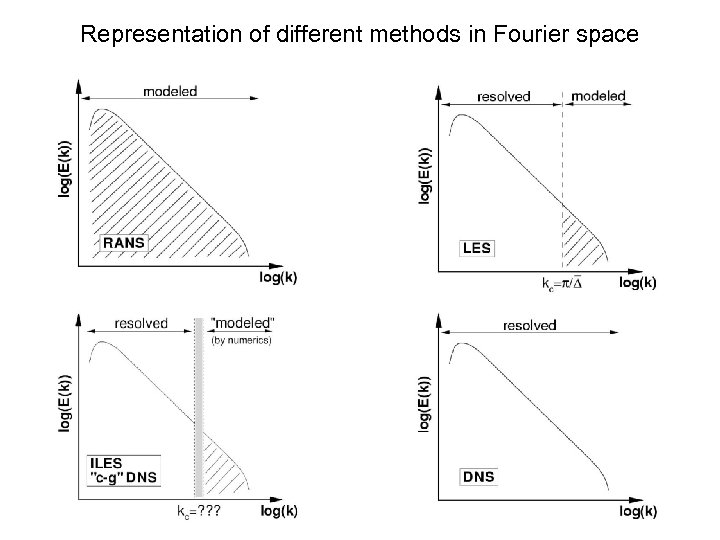Representation of different methods in Fourier space 11

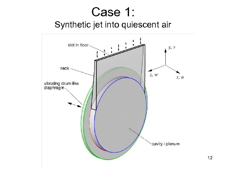Case 1: Synthetic jet into quiescent air 12

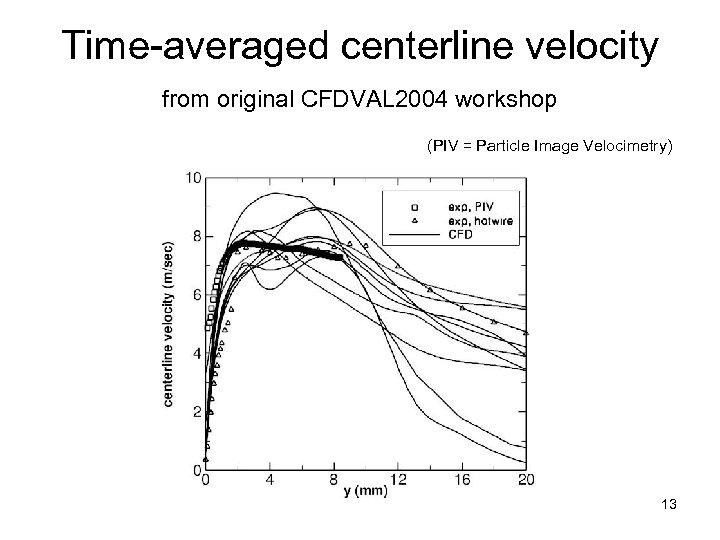Time-averaged centerline velocity from original CFDVAL 2004 workshop (PIV = Particle Image Velocimetry) 13

Analysis • Workshop CFD results “all over the map” – Turb models and slot BCs had big impact • Experiment PIV & hotwire different near slot in original experiment – New experiment (post-workshop) - at slightly different conditions – New experiment PIV & Laser Doppler Velocimetry (LDV) agreed well – Hotwire not accurate near slot 14

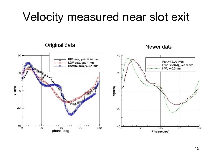Velocity measured near slot exit Original data Newer data 15

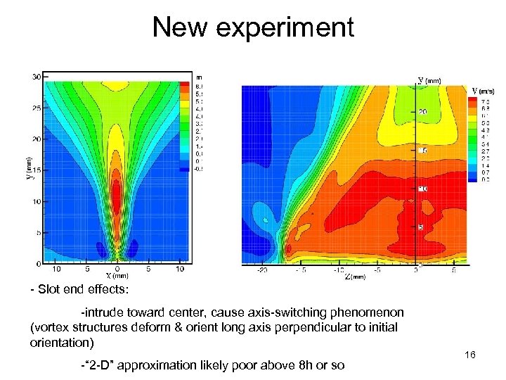New experiment - Slot end effects: -intrude toward center, cause axis-switching phenomenon (vortex structures deform & orient long axis perpendicular to initial orientation) -“ 2 -D” approximation likely poor above 8 h or so 16

Published results for case 1 • Yamaleev & Carpenter - low-order (1 -D Euler) method for internal cavity coupled to laminar flow N-S in field • Vatsa & Turkel - URANS with FFT curve fitting of internal slot BC to match flow at exit • Zhang & Wang - URANS with similar FFT internal BC • Park et al - URANS with internal BC curve fit to data • Carpy & Manceau - URANS with no cavity; exp data at exit used for BC • Xia & Qin - DES with predictive moving wall internal BC • Cui & Agarwal - DES & SST-LES; simple sinusoidal internal BC to try to match PIV & hotwire • Kotapati et al - N-S; simple sinusoidal internal BC to try to match PIV 17

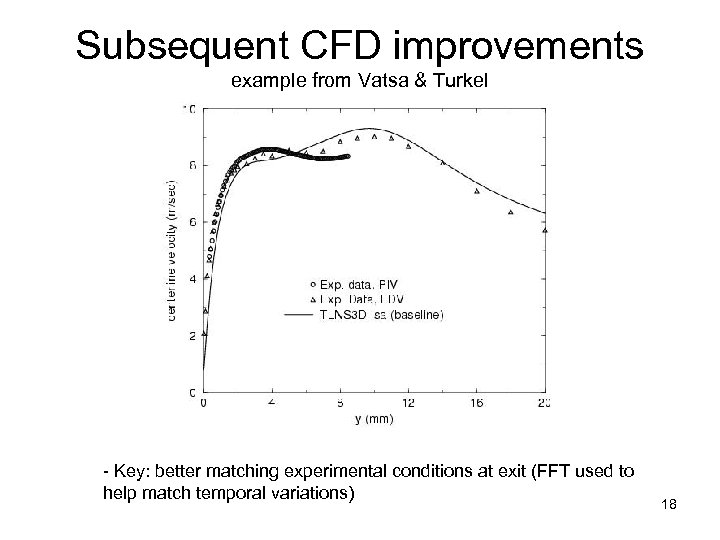Subsequent CFD improvements example from Vatsa & Turkel - Key: better matching experimental conditions at exit (FFT used to help match temporal variations) 18

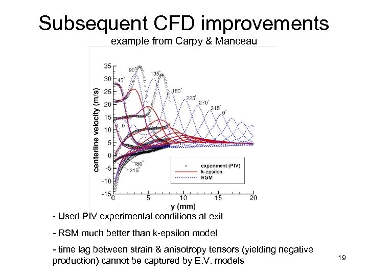Subsequent CFD improvements example from Carpy & Manceau - Used PIV experimental conditions at exit - RSM much better than k-epsilon model - time lag between strain & anisotropy tensors (yielding negative production) cannot be captured by E. V. models 19

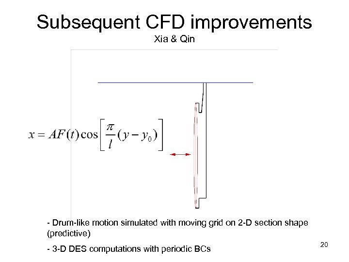Subsequent CFD improvements Xia & Qin - Drum-like motion simulated with moving grid on 2 -D section shape (predictive) - 3 -D DES computations with periodic BCs 20

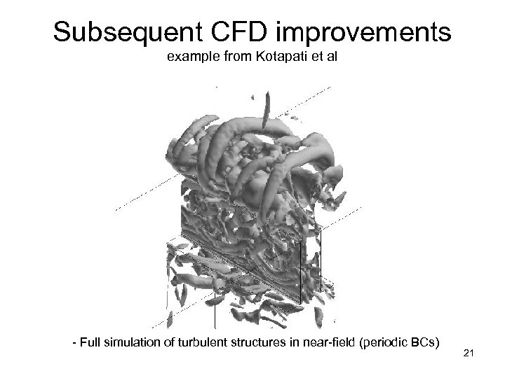Subsequent CFD improvements example from Kotapati et al - Full simulation of turbulent structures in near-field (periodic BCs) 21

Summary - case 1 • What’s new – Recognition of importance of end effects – Development/recognition of techniques to better match BCs at exit – Internal cavity shape itself not a major factor • But you need exp data at exit to match • Predictive modeling of membrane motion used 2 -D version of actual cavity shape – DES and N-S simulations (as well as URANS) have been successful in the near-field 22

Summary - case 1 • Remaining challenges – Unclear whether URANS is adequate & which models are best • SA & SST appear reasonable, but Carpy & Manceau suggest linear models miss key physics • When is simulation (e. g. , DES, N-S) necessary? – Capturing 3 -D end effects (and physics further into the field) possible? – How well will a predictive moving-grid BC for 3 -D diaphragm shape work? 23

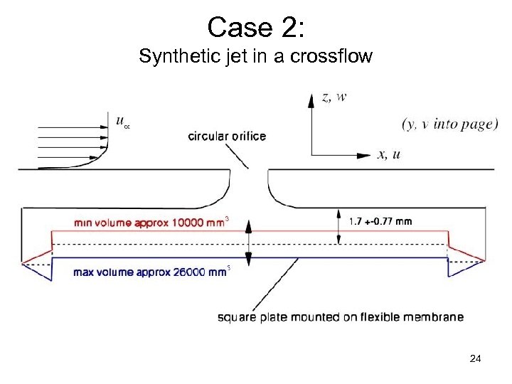Case 2: Synthetic jet in a crossflow 24

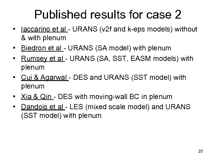Published results for case 2 • Iaccarino et al - URANS (v 2 f and k-eps models) without & with plenum • Biedron et al - URANS (SA model) with plenum • Rumsey et al - URANS (SA, SST, EASM models) with plenum • Cui & Agarwal - DES and URANS (SST model) with plenum • Xia & Qin - DES with moving-wall BC in plenum • Dandois et al - LES (mixed scale model) and URANS (SST model) with plenum 25

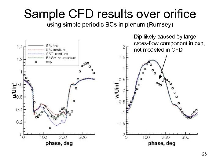Sample CFD results over orifice using simple periodic BCs in plenum (Rumsey) Dip likely caused by large cross-flow component in exp, not modeled in CFD 26

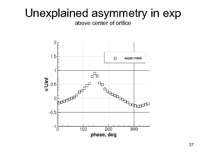Unexplained asymmetry in exp above center of orifice 27

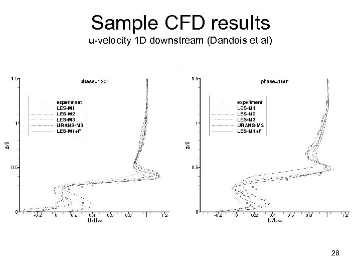Sample CFD results u-velocity 1 D downstream (Dandois et al) 28

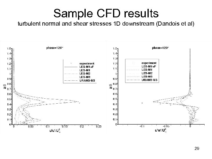Sample CFD results turbulent normal and shear stresses 1 D downstream (Dandois et al) 29

Summary - case 2 • What’s new – LES (with appropriate upstream inflow BCs) better than URANS at predicting turbulent quantities • Earlier: recognition at CFDVAL 2004 workshop that URANS & LES could both predict mean flow quantities reasonably well – Including orifice important for capturing complex flowfield in its immediate vicinity • Simple top-hat wall BCs miss physics – Dandois demonstrated potential effects of large periodic cross-flow velocity component in experiment – Xia & Qin used moving wall BC in plenum • Results appeared to be similar to usual simple periodic transpiration BC 30

Summary - case 2 • Remaining challenges – Can a predictive (moving wall) BC in plenum be used to achieve closer agreement with velocities at orifice exit? – In light of unexplained large v-velocity component in workshop experiment, revisit experiment or establish new benchmark dataset 31

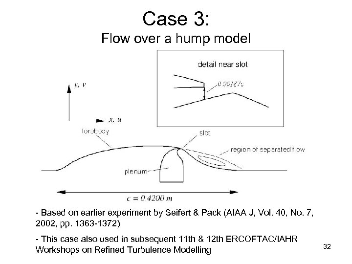Case 3: Flow over a hump model - Based on earlier experiment by Seifert & Pack (AIAA J, Vol. 40, No. 7, 2002, pp. 1363 -1372) - This case also used in subsequent 11 th & 12 th ERCOFTAC/IAHR Workshops on Refined Turbulence Modelling 32

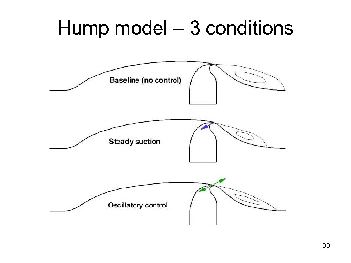Hump model – 3 conditions 33

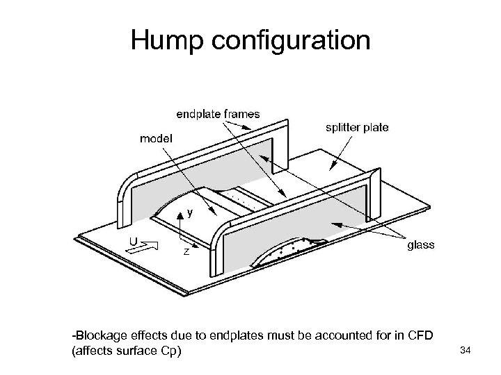Hump configuration -Blockage effects due to endplates must be accounted for in CFD (affects surface Cp) 34

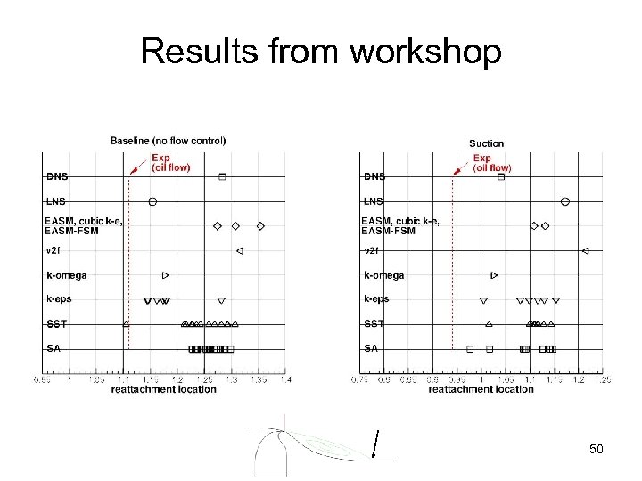
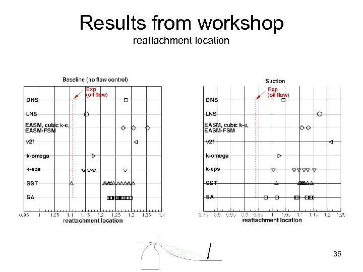Results from workshop reattachment location 35

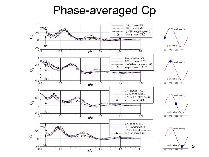Phase-averaged Cp 36

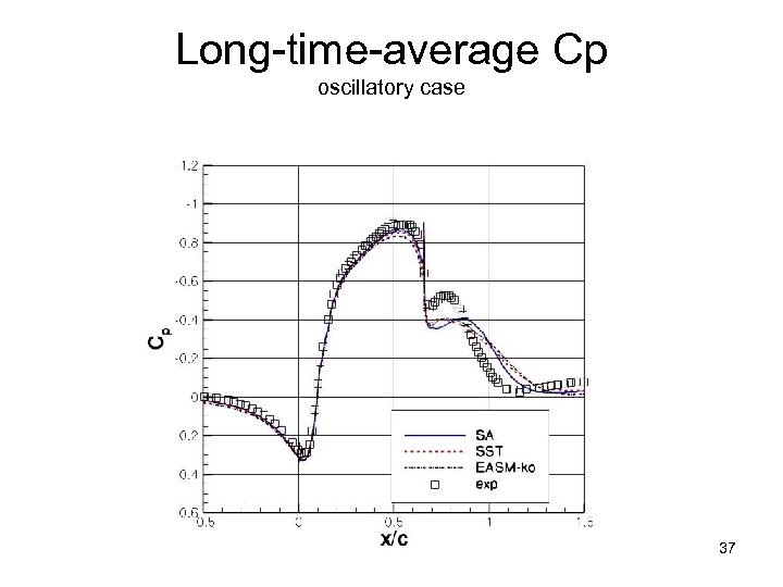Long-time-average Cp oscillatory case 37

RANS/URANS problem identified • Eddy viscosity underpredicted in separated shear layer region – Too little mixing – Too late a reattachment downstream – Occurs for baseline, steady suction, or oscillatory control – Similar problem seen in a separate 2 -D hill workshop case • Hump case has been computed by no less than 16 different groups 38

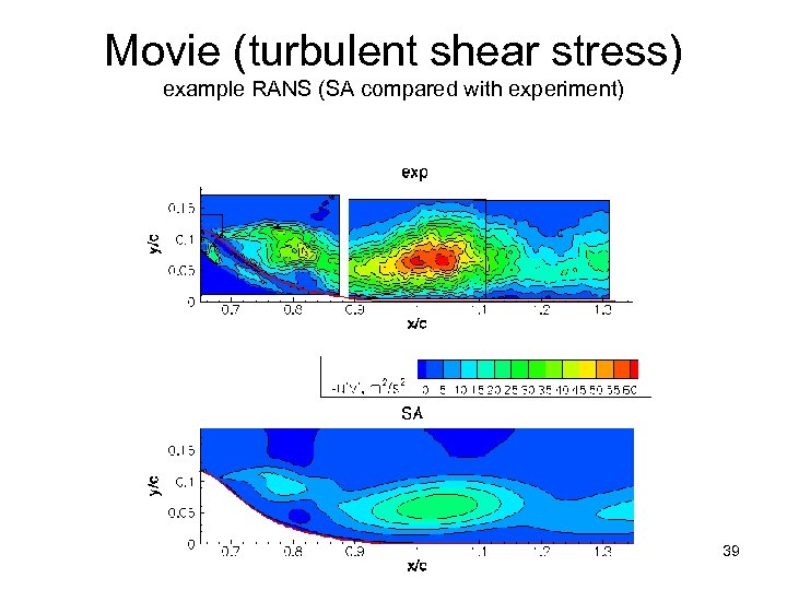Movie (turbulent shear stress) example RANS (SA compared with experiment) 39

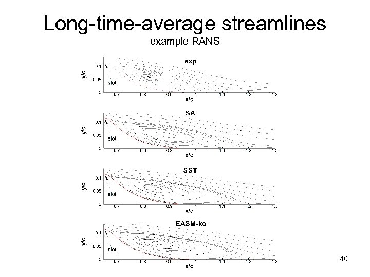Long-time-average streamlines example RANS 40

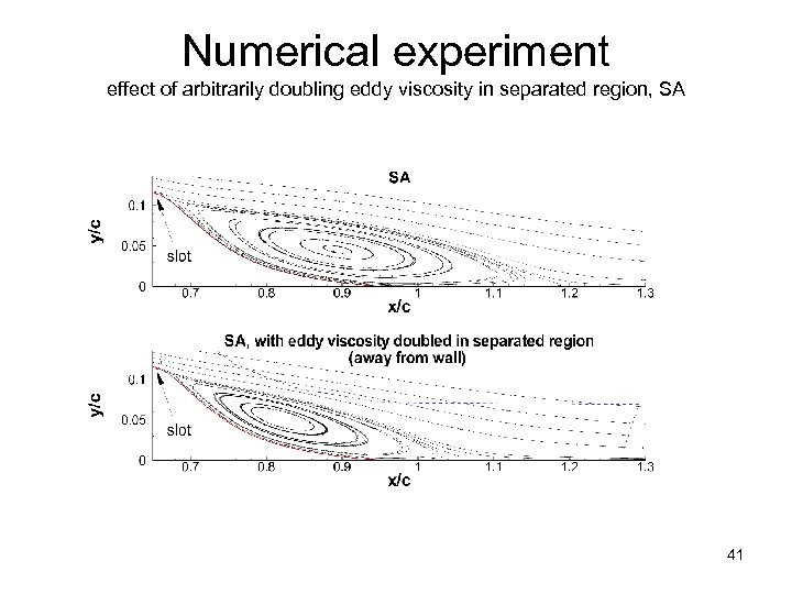Numerical experiment effect of arbitrarily doubling eddy viscosity in separated region, SA 41

RANS/URANS results for case 3 • • Iaccarino et al Capizzano et al - used Neumann surface BCs Cui & Agarwal Balakumar - employed higher order WENO Morgan et al - employed higher order compact scheme Bettini & Cravero - commercial package He et al - commercial package; looked at plasma control – k-epsilon attached earlier – but because it separated later, not due to better physics! • Madugundi et al - commercial package • Rumsey et al - included parametric studies at other conditions from the experiment 42

Blended RANS-LES, & DNS • Israel et al - EASM combined with FSM • Hiller & Seitz - SAS model • Krishnan et al - DES – Also RANS with many variants, including 3 -D with endplates – Helped discover blockage issues • Biswas - LES (dynamic model with KE eqn) • Saric et al - LES (Smagorinsky - const Cs), DES, and RANS • Morgan et al - ILES • You et al - LES (dynamic Smagorinsky) • Franck & Colonius - LES (both types Smag) & ILES • Postl & Fasel - “coarse-grid” DNS 43

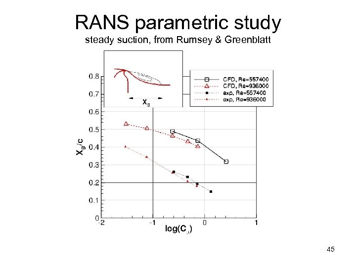
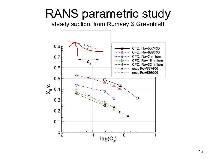
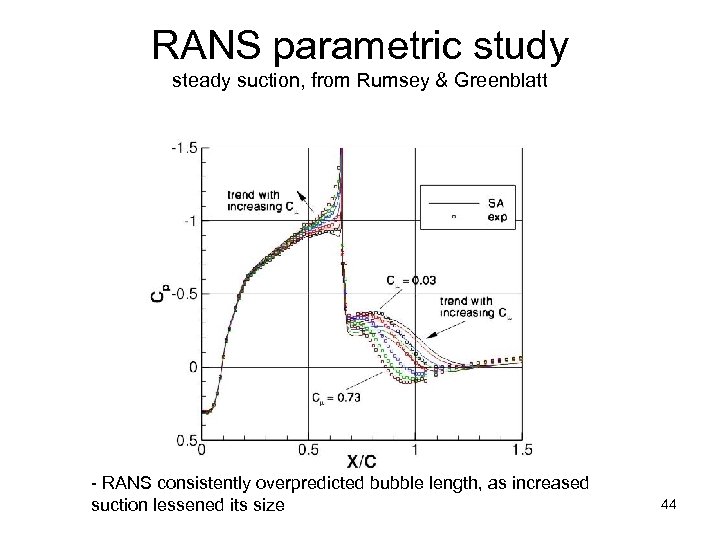RANS parametric study steady suction, from Rumsey & Greenblatt - RANS consistently overpredicted bubble length, as increased suction lessened its size 44

RANS parametric study steady suction, from Rumsey & Greenblatt 45

RANS parametric study steady suction, from Rumsey & Greenblatt 46

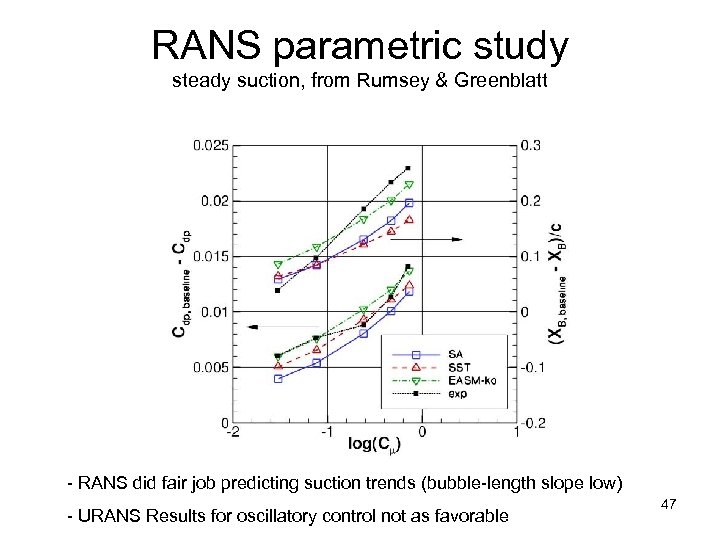RANS parametric study steady suction, from Rumsey & Greenblatt - RANS did fair job predicting suction trends (bubble-length slope low) - URANS Results for oscillatory control not as favorable 47

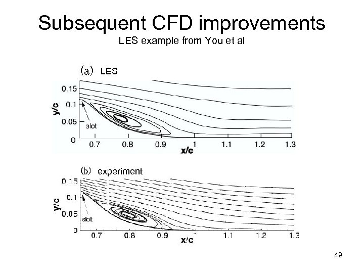
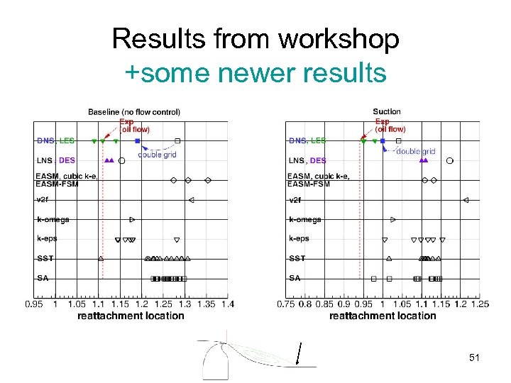
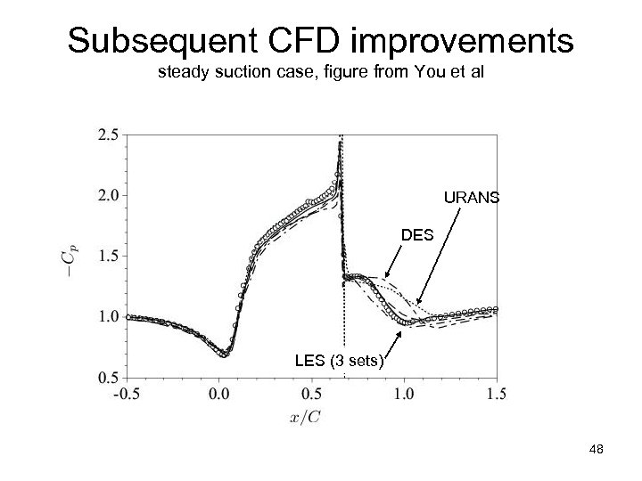Subsequent CFD improvements steady suction case, figure from You et al URANS DES LES (3 sets) 48

Subsequent CFD improvements LES example from You et al LES experiment 49

Results from workshop 50

Results from workshop +some newer results 51

Summary - case 3 • What’s new – RANS/URANS • Trends for steady suction can be obtained in fair agreement with experimental trends (oscillatory control not so good) • Can get right answer (bubble length) for wrong reason with kepsilon, for example • Computing with or without plenum not a big factor when looking at global flow field properties – DES • Shown to work well for baseline case • Generally no benefit for smaller bubbles (issues related to RANS-LES interface location and insufficient eddy content) – LES & coarse-grid DNS • Can yield very good results 52

Summary - case 3 • Remaining challenges – Is there bubble size small enough for which RANS/URANS predicts physics & reattachment well? – Improve blended RANS-LES methods like DES to work more consistently, especially for cases with small separations – How well can LES predict trends due to jet strength, Re, frequency, etc? – Can LES-type simulations be used to help improve RANS/URANS models for this class of flows? 53

Conclusions • CFD increasingly called upon to predict synthetic-jet flows • Need to establish confidence in CFD – Through verification/validation studies and records of documented successes & failures • Workshops such as CFDVAL 2004 are an important part of this documentation 54

Important to “follow through” and address challenges that remain - additional follow-up flow control CFD workshops would be useful 55

End 56

Backup slides 57

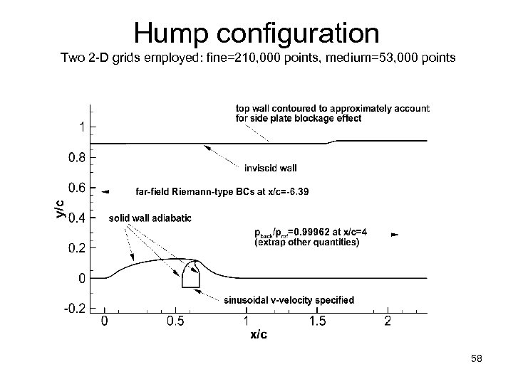Hump configuration Two 2 -D grids employed: fine=210, 000 points, medium=53, 000 points 58

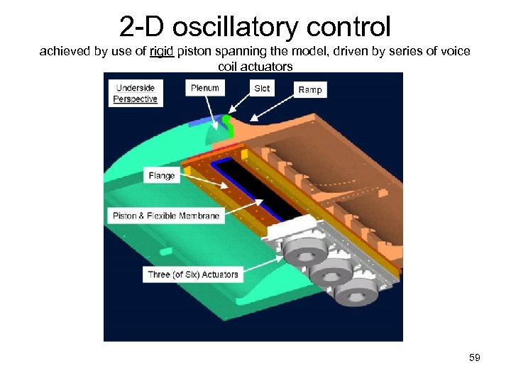2 -D oscillatory control achieved by use of rigid piston spanning the model, driven by series of voice coil actuators 59

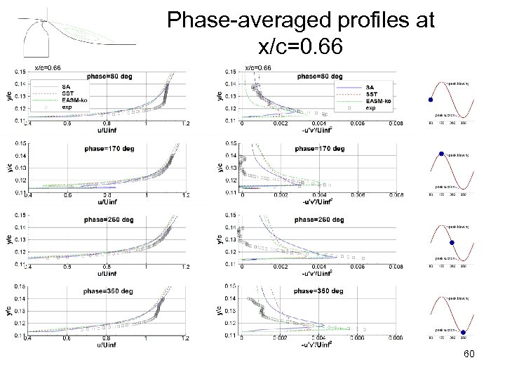Phase-averaged profiles at x/c=0. 66 60

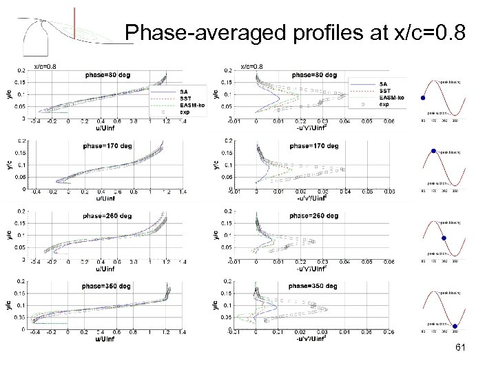Phase-averaged profiles at x/c=0. 8 61

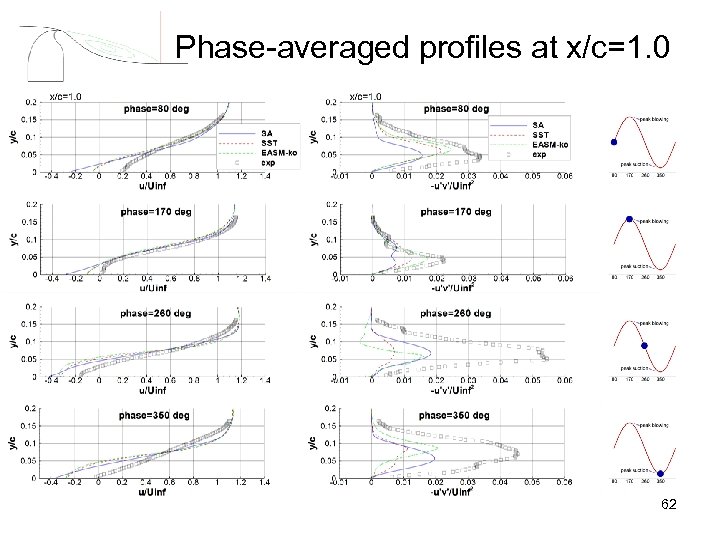Phase-averaged profiles at x/c=1. 0 62