String Processing II Compressed Indexes Patrick Nichols pnichols mit

String Processing II: Compressed Indexes Patrick Nichols (pnichols@mit. edu) Jon Sheffi (jsheffi@mit. edu) Dacheng Zhao (zhao@mit. edu) Compressed Indexes - Nichols, Sheffi, Zhao

The Big Picture • We’ve seen ways of using complex data structures (suffix arrays and trees) to perform character string queries • The Burrows and Wheeler (BWT) transform is a reversible operation used on suffix arrays • Compression on transformed suffix arrays improves performance Compressed Indexes - Nichols, Sheffi, Zhao 2

Lecture Outline • • • Motivation and compression Review of suffix arrays The BW transform (to and from) Searching in compressed indexes Conclusion Questions Compressed Indexes - Nichols, Sheffi, Zhao 3

Motivation • Most interesting massive data sets contain string data (the web, human genome, digital libraries, mailing lists) • There are incredible amounts of textual data out there (~1000 TB) (Ferragina) • Performing high speed queries on such material is critical for many applications Compressed Indexes - Nichols, Sheffi, Zhao 4

Why Compress Data? • Compression saves space (though disks are getting cheaper -- < $1/GB) • I/O bottlenecks and Moore’s law make CPU operations “free” • Want to minimize seeks and reads for indexes too large to fit in main memory • More on compression in lecture 21 Compressed Indexes - Nichols, Sheffi, Zhao 5

Background • Last time, we saw the suffix array, which provides pointers to the ordered suffixes of a string T. T = ababc T[1] = ababc T[3] = abc T[2] = babc T[4] = bc A = [1 3 2 4 5] Each entry in A tells us what the lexographic order of the ith substring is. T[5] = c Compressed Indexes - Nichols, Sheffi, Zhao 6

Background • What’s wrong with suffix trees and arrays? • They use O(N log N) + N log |Σ| bits (array of N numbers + text, assuming alphabet Σ). This could be much more than the size of the uncompressed text, since usually log N = 32 and log |Σ| = 8. • We can use compression to use less space in linear time! Compressed Indexes - Nichols, Sheffi, Zhao 7

BW-Transform • Why BWT? We can use the BWT to compress T in a provably optimal manner, using O(Hk(T)) + o(1) bits per input symbol in the worst case, where Hk(T) is the kth order empirical entropy. • What is Hk? Hk is the maximum compression we can achieve using for each character a code which depends on the k characters preceding it. Compressed Indexes - Nichols, Sheffi, Zhao 8

The BW-Transform 1. Start with text T. Append # character, which is lexicographically before all other characters in the alphabet, Σ. 2. Generate all of the cyclic shifts of T# and sort them lexicographically, forming a matrix M with rows and columns equal to |T#| = |T| + 1. 3. Construct L, the transformed text of T, by taking the last column of M. Compressed Indexes - Nichols, Sheffi, Zhao 9

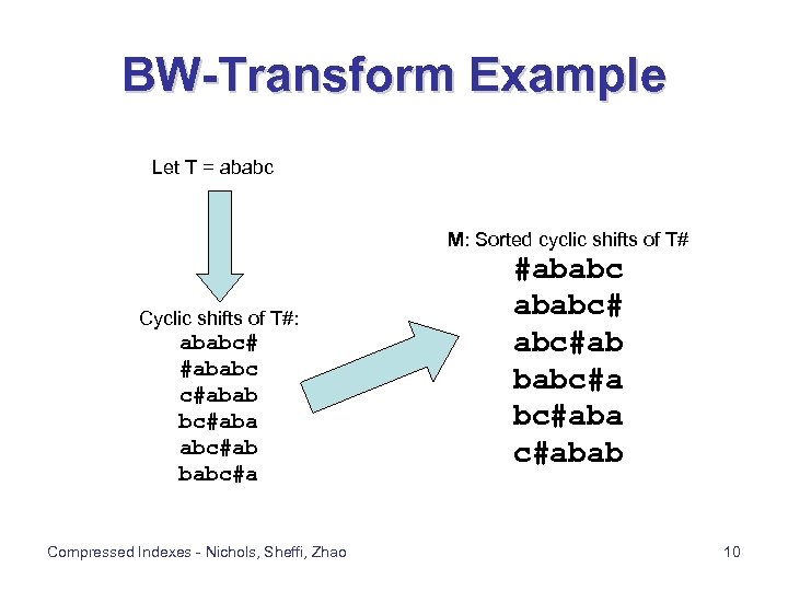BW-Transform Example Let T = ababc M: Sorted cyclic shifts of T# Cyclic shifts of T#: ababc# #ababc c#abab bc#aba abc#ab babc#a Compressed Indexes - Nichols, Sheffi, Zhao #ababc# abc#ab babc#aba c#abab 10

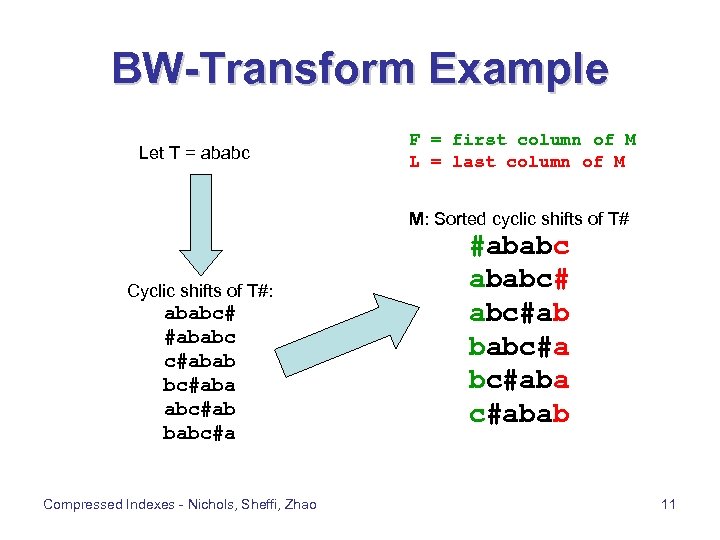BW-Transform Example Let T = ababc F = first column of M L = last column of M M: Sorted cyclic shifts of T# Cyclic shifts of T#: ababc# #ababc c#abab bc#aba abc#ab babc#a Compressed Indexes - Nichols, Sheffi, Zhao #ababc# abc#ab babc#aba c#abab 11

Inverse BW-Transform • Construct C[1…|Σ|], which stores in C[c] the cumulative number of occurrences in T of characters 1 through c-1. • Construct an LF-mapping LF[1…|T|+1] which maps each character to the character occurring previously in T using only L and C. • Reconstruct T backwards by threading through the LF-mapping and reading the characters off of L. Compressed Indexes - Nichols, Sheffi, Zhao 12

Inverse BW-Transform: Construction of C • Store in C[c] the number of occurrences in T# of the characters {#, 1, …, c-1}. • In our example: T# = ababc# 1 #, 2 a, 2 b, 1 c # a b c C = [0 1 3 5] • Notice that C[c] + n is the position of the nth occurrence of c in F (if any). Compressed Indexes - Nichols, Sheffi, Zhao 13

Inverse BW-Transform: Constructing the LF-mapping • Why and how the LF-mapping? Notice that for every row of M, L[i] directly precedes F[i] in the text (thanks to the cyclic shifts). • Let L[i] = c, let ri be the number of occurrences of c in the prefix L[1, i], and let M[j] be the ri-th row of M that starts with c. Then the character in the first column F corresponding to L[i] is located at F[j]. • How to use this fact in the LF-mapping? Compressed Indexes - Nichols, Sheffi, Zhao 14

Inverse BW-Transform: Constructing the LF-mapping • So, define LF[1…|T|+1] as LF[i] = C[L[i]] + ri. • C[L[i]] gets us the proper offset to the zeroth occurrence of L[i], and the addition of ri gets us the ri-th row of M that starts with c. Compressed Indexes - Nichols, Sheffi, Zhao 15

Inverse BW-Transform: Constructing the LF-mapping LF[1] LF[2] LF[3] LF[4] LF[5] LF[6] LF[i] = C[L[i]] + ri = C[L[1]] + 1 = 5 = C[L[2]] + 1 = 0 = C[L[3]] + 1 = 3 = C[L[4]] + 1 = C[L[5]] + 2 = 1 = C[L[6]] + 2 = 3 LF[] = [6 1 4 2 3 Compressed Indexes - Nichols, Sheffi, Zhao + 1 + 1 + 2 5] = = = 6 1 4 2 3 5 16

Inverse BW-Transform: Reconstruction of T • Start with T[] blank. Let u = |#T| Initialize s = 1 and T[u] = L[1]. We know that L[1] is the last character of T because M[1] = #T. • For each i = u-1, …, 1 do: s = LF[s] (threading backwards) T[i] = L[s] (read off the next letter back) Compressed Indexes - Nichols, Sheffi, Zhao 17

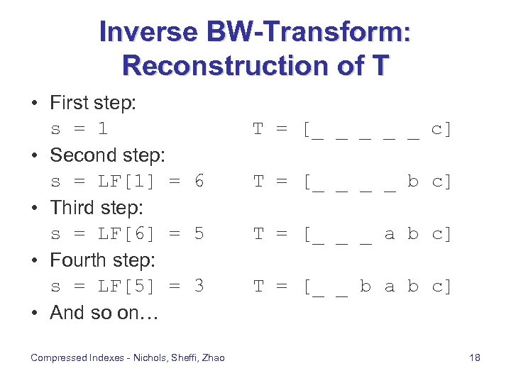Inverse BW-Transform: Reconstruction of T • First step: s = 1 • Second step: s = LF[1] = 6 • Third step: s = LF[6] = 5 • Fourth step: s = LF[5] = 3 • And so on… Compressed Indexes - Nichols, Sheffi, Zhao T = [_ _ _ c] T = [_ _ b c] T = [_ _ _ a b c] T = [_ _ b a b c] 18

BW Transform Summary • The BW transform is reversible • We can construct it in O(n) time • We can reverse it to reconstruct T in O(n) time, using O(n) space • Once we obtain L, we can compress L in a provably efficient manner Compressed Indexes - Nichols, Sheffi, Zhao 19

So, what can we do with compressed data? • It’s compressed, hence saving us space; to search, simply decompress and search • Search for the number of occurrences in the compressed (mostly compressed) data. • Locate where the occurrences are in the original string from the compressed (mostly compressed) data. Compressed Indexes - Nichols, Sheffi, Zhao 20

BWT_count Overview • BWT_count begins with the last character of the query (P[1, p]) and works forwards • Simplistically, BWT_count looks for the suffixes of P[1, p]. If a suffix of P[1, p] is not in T, quit. • Running time is O(p) because running time of Occ(c, 1, k) is O(1) • space needed = L compressed + space needed by Occ() = L compressed L + O((u / log u) Compressed Indexes - Nichols, Sheffi, Zhao 21

Searching BWT-compressed text: Algorithm BW_count(P[1, p]) 1. c = P[p], i = p 2. sp = C[c] + 1, ep = C[c+1] 3. while ((sp ep)) and (i 2)) do 4. c = P[i-1] 5. sp = C[c] + Occ(c, 1, sp – 1) + 1 6. ep = C[c] + Occ(c, 1, ep) 7. i = i - 1 8. if (ep < sp) then return “pattern” not found else return “found (ep – sp + 1) occurrences” Occ(c, 1, k) finds the number of occurrences of c in the range 1 to k in L Invariant: at the i-th stage, sp points at the first row of M prefixed by P[i, p] and ep points to the last row of M prefixed by P[i, p]. Compressed Indexes - Nichols, Sheffi, Zhao 22

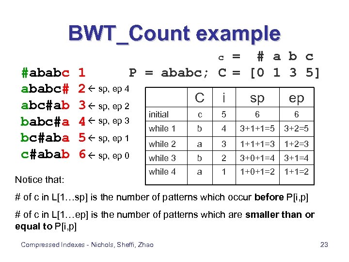BWT_Count example = # a b c P = ababc; C = [0 1 3 5] c #ababc# abc#ab babc#aba c#abab Notice that: 1 2 sp, ep 4 3 sp, ep 2 4 sp, ep 3 5 sp, ep 1 6 sp, ep 0 C i sp ep initial c 5 6 6 while 1 b 4 3+1+1=5 3+2=5 while 2 a 3 1+1+1=3 1+2=3 while 3 b 2 3+0+1=4 3+1=4 while 4 a 1 1+0+1=2 1+1=2 # of c in L[1…sp] is the number of patterns which occur before P[i, p] # of c in L[1…ep] is the number of patterns which are smaller than or equal to P[i, p] Compressed Indexes - Nichols, Sheffi, Zhao 23

Running Time of Occ(c, 1, k) • We can do this trivially O(logk) with augmented B trees by exploiting the continuous runs in L – One tree per character – Nodes store ranges and total number of said character in that range • By exploiting other techniques, we can reduce time to O(1) Compressed Indexes - Nichols, Sheffi, Zhao 24

Locating the Occurrences • Naïve solution: Use BWT_count to find number of occurrences and also sp and ep. Uncompress L, untransform M and calculate the position of the occurrence in the string. • Better solution (time O(p + occ log 2 u), space O(u / log u): 1. preprocess M by logically marking rows in M which correspond to text positions (1 + i • n), where n = θ(log 2 u), and i = 0, 1, … , u/n 2. to find pos(s), if s is marked, done; otherwise, use LF to find row s’ corresponding to the suffix T[pos(s) – 1, u]. Iterate v times until s’ points to a marked row; pos(s) = pos(s’) + v • Best solution (time O(p + occlogε u), space …): Refine the better solution so that we still mark rows but we also have “shortcuts” so that we can jump by more than one character at a time Compressed Indexes - Nichols, Sheffi, Zhao 25

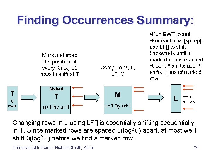Finding Occurrences Summary: Mark and store the position of every θ(log 2 u), rows in shifted T T U rows Shifted Compute M, L, LF, C T M u+1 by u+1 • Run BWT_count • For each row [sp, ep], use LF[] to shift backwards until a marked row is reached • Count # shifts; add # shifts + pos of marked row L sp ep Changing rows in L using LF[] is essentially shifting sequentially in T. Since marked rows are spaced θ(log 2 u) apart, at most we’ll shift θ(log 2 u) before we find a marked row. Compressed Indexes - Nichols, Sheffi, Zhao 26

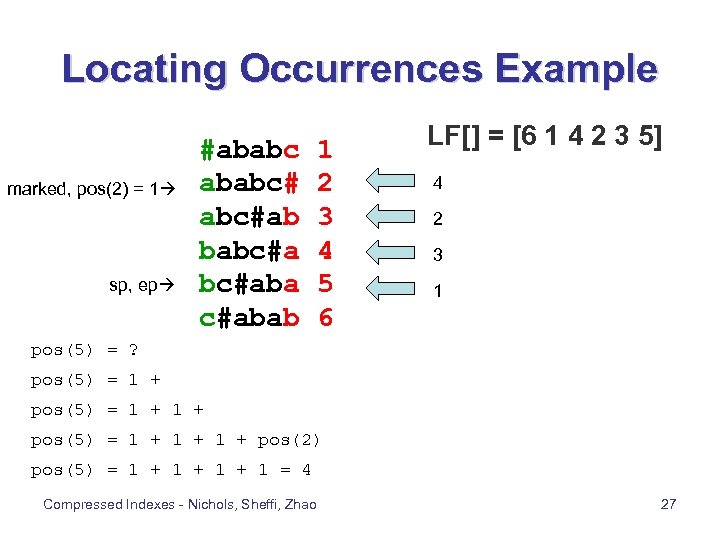Locating Occurrences Example marked, pos(2) = 1 sp, ep #ababc# abc#ab babc#aba c#abab 1 2 3 4 5 6 LF[] = [6 1 4 2 3 5] 4 2 3 1 pos(5) = ? pos(5) = 1 + 1 + pos(2) pos(5) = 1 + 1 + 1 = 4 Compressed Indexes - Nichols, Sheffi, Zhao 27

Conclusions • Free CPU operations make compression a great idea, given I/O bottlenecks • The BW transform makes the index more amenable to compression • We can perform string queries on a compressed index without any substantial performance loss Compressed Indexes - Nichols, Sheffi, Zhao 28

Questions? • Any questions? Compressed Indexes - Nichols, Sheffi, Zhao 29