Strategy and Sales Program Planning Topic 2 Cont

Strategy and Sales Program Planning Topic 2 Cont….

Estimating Potentials & Forecasting Sales n n n Key to success in sales is knowing where customers are located & being able to predict how much they will buy. Market potential – is an estimate of maximum demand in a time period based on the number of potential users & the purchase rate. Some of the methods of sales forecasting (qualitative & quantitative) are sales force composite, jury of executive opinion, intention to buy survey, moving average, exponential smoothing, simple & multiple regression.

Qualitative: 1. Sales Force Composite Sales people project volume for customers in their own territory & estimates are aggregated & reviewed at higher mgt level. n Mostly practiced by industrial companies due to limited number of customers sales people are in a good position to assess customers needs. n

2. Jury of Executive Opinion Soliciting judgment of a group of experienced managers to give sales estimates for new & current products. n It is fast & allows inclusion of subjective factors such as competition, economic climate, weather & union activity. n

Quantitative: 1. Seasonal Adjustments Sales forecasts are often prepared monthly or quarterly. n Collect sales figures for past several years need to be used. n Sales for months/quarters are averaged across years to build a seasonal index. n Then index are developed. n Next computer programs are used to do sales forecasting for the companies. n

2. Moving Averages The average revenue achieved over several periods is used as a prediction of sales in the next period. n Assumes the future will be an average of the past achievements. n

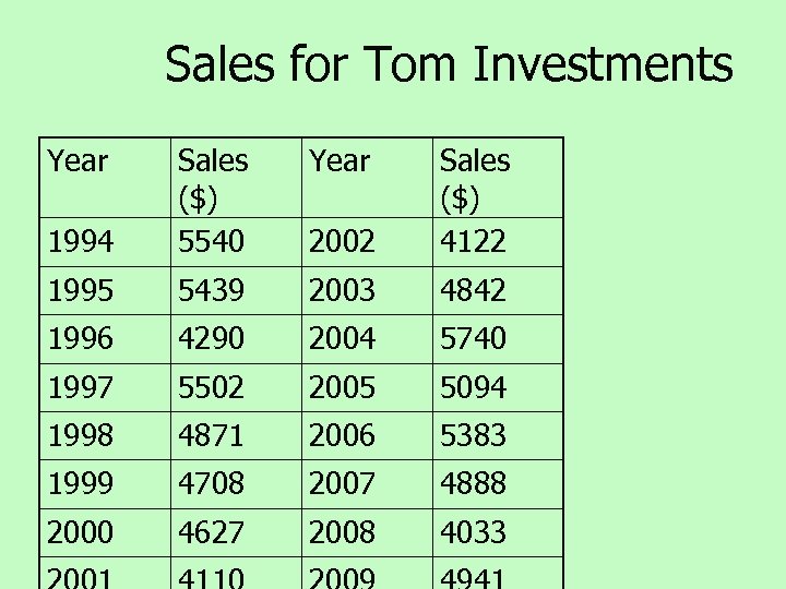Sales for Tom Investments Year 1994 Sales ($) 5540 2002 Sales ($) 4122 1995 5439 2003 4842 1996 4290 2004 5740 1997 5502 2005 5094 1998 4871 2006 5383 1999 4708 2007 4888 2000 4627 2008 4033

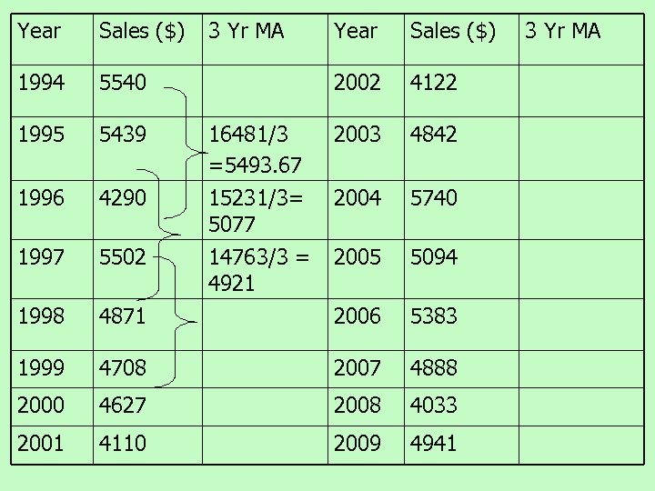Year Sales ($) 1994 5540 1995 5439 1996 3 Yr MA Year Sales ($) 2002 4122 16481/3 =5493. 67 2003 4842 4290 15231/3= 5077 2004 5740 1997 5502 14763/3 = 4921 2005 5094 1998 4871 2006 5383 1999 4708 2007 4888 2000 4627 2008 4033 2001 4110 2009 4941 3 Yr MA

n n n n In the earlier example you need to take 3 values at a time average it, First 3 years, Then take yr 2, 3, 4 average and write answer. And so on till you complete the rest. Plot the graph of 1) year on x-axis, sales Y-axis. On the same graph plot year on axis, moving average on Y axis. Compare the two graphs Moving average is more smoother. This is because the fluctuations have been adjusted.

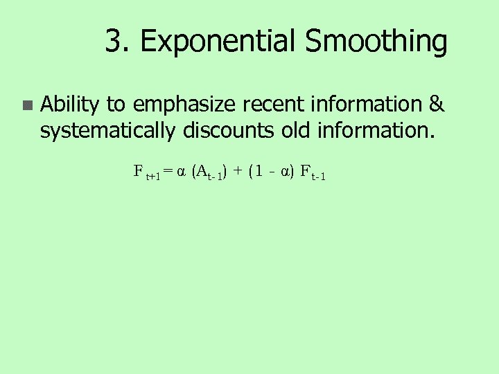3. Exponential Smoothing n Ability to emphasize recent information & systematically discounts old information. F t+1 = (At-1) + (1 - ) Ft-1

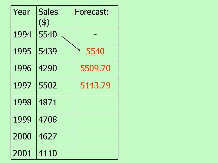
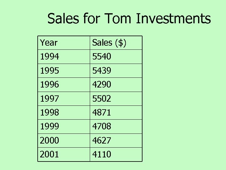Sales for Tom Investments Year Sales ($) 1994 5540 1995 5439 1996 4290 1997 5502 1998 4871 1999 4708 2000 4627 2001 4110

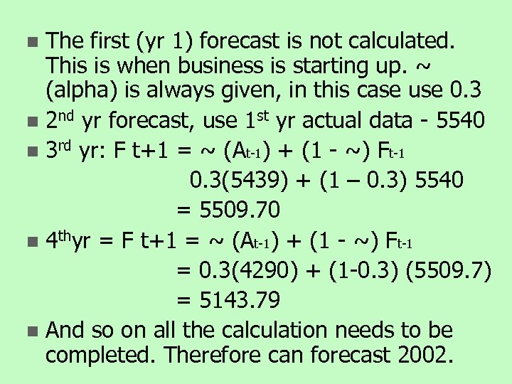The first (yr 1) forecast is not calculated. This is when business is starting up. ~ (alpha) is always given, in this case use 0. 3 n 2 nd yr forecast, use 1 st yr actual data - 5540 n 3 rd yr: F t+1 = ~ (At-1) + (1 - ~) Ft-1 0. 3(5439) + (1 – 0. 3) 5540 = 5509. 70 n 4 thyr = F t+1 = ~ (At-1) + (1 - ~) Ft-1 = 0. 3(4290) + (1 -0. 3) (5509. 7) = 5143. 79 n And so on all the calculation needs to be completed. Therefore can forecast 2002. n

Year Sales ($) 1994 5540 Forecast: - 1995 5439 5540 1996 4290 5509. 70 1997 5502 5143. 79 1998 4871 1999 4708 2000 4627 2001 4110

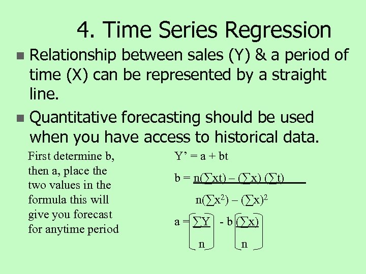4. Time Series Regression Relationship between sales (Y) & a period of time (X) can be represented by a straight line. n Quantitative forecasting should be used when you have access to historical data. n First determine b, then a, place the two values in the formula this will give you forecast for anytime period Y’ = a + bt b = n(∑xt) – (∑x) (∑t) n(∑x 2) – (∑x)2 a = ∑Y - b (∑x) n n

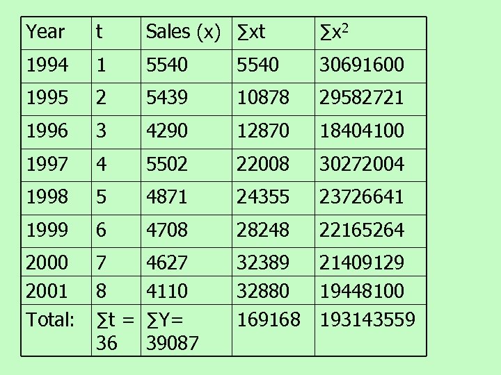Year t Sales (x) ∑xt ∑x 2 1994 1 5540 30691600 1995 2 5439 10878 29582721 1996 3 4290 12870 18404100 1997 4 5502 22008 30272004 1998 5 4871 24355 23726641 1999 6 4708 28248 22165264 2000 2001 Total: 7 8 ∑t = 36 4627 4110 ∑Y= 39087 32389 21409129 32880 19448100 169168 193143559

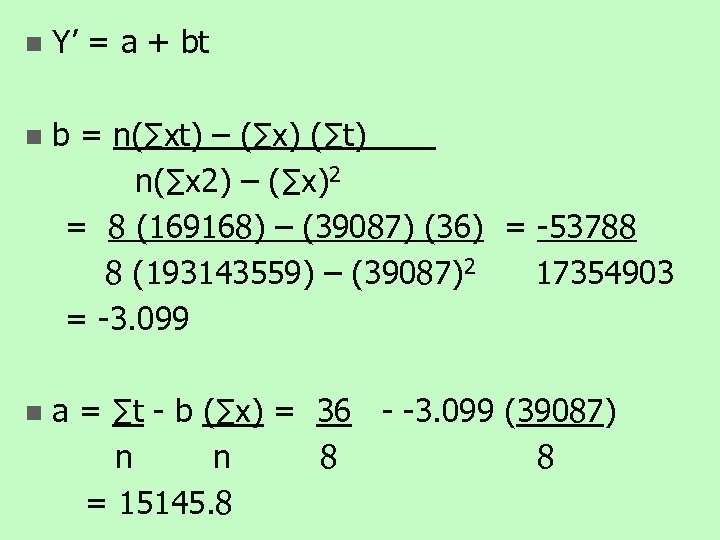n Y’ = a + bt n b = n(∑xt) – (∑x) (∑t) n(∑x 2) – (∑x)2 = 8 (169168) – (39087) (36) = -53788 8 (193143559) – (39087)2 17354903 = -3. 099 n a = ∑t - b (∑x) = 36 - -3. 099 (39087) n n 8 8 = 15145. 8

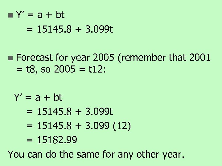n Y’ = a + bt = 15145. 8 + 3. 099 t n Forecast for year 2005 (remember that 2001 = t 8, so 2005 = t 12: Y’ = a + bt = 15145. 8 + 3. 099 (12) = 15182. 99 You can do the same for any other year.