Stochastic Optimization is almost as easy as Deterministic

Stochastic Optimization is (almost) as easy as Deterministic Optimization Chaitanya Swamy Joint work with David Shmoys done while at Cornell University

Stochastic Optimization • Way of modeling uncertainty. • Exact data is unavailable or expensive – data is uncertain, specified by a probability distribution. • Want to make the best decisions given this uncertainty in the data. Applications in logistics, transportation models, financial instruments, network design, production planning, … • Dates back to 1950’s and the work of Dantzig.

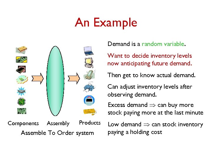An Example Demand is a random variable. Want to decide inventory levels now anticipating future demand. Then get to know actual demand. Can adjust inventory levels after observing demand. Excess demand Þ can buy more stock paying more at the last minute Components Assembly Products Assemble To Order system Low demand Þ can stock inventory paying a holding cost

Two-Stage Recourse Model Given : Probability distribution over inputs. Stage I : Make some advance decisions – plan ahead or hedge against uncertainty. Observe the actual input scenario. Stage II : Take recourse. Can augment earlier solution paying a Choose cost. recoursestage I decisions to minimize (stage I cost) + (expected stage II recourse cost).

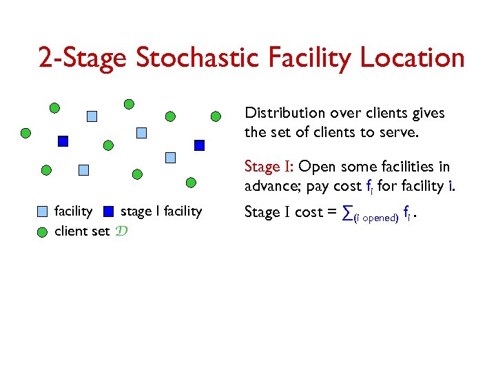2 -Stage Stochastic Facility Location Distribution over clients gives the set of clients to serve. Stage I: Open some facilities in advance; pay cost fi for facility i. facility stage I facility client set D Stage I cost = ∑(i opened) fi.

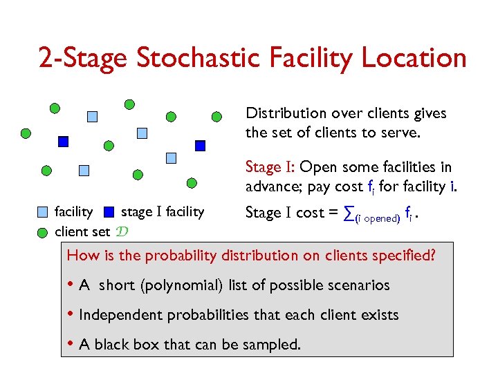2 -Stage Stochastic Facility Location Distribution over clients gives the set of clients to serve. Stage I: Open some facilities in advance; pay cost fi for facility i. facility stage I facility client set D Stage I cost = ∑(i opened) fi. How is the probability distribution on clients specified? • A short (polynomial) list of possible scenarios • Independent probabilities that each client exists • A black box that can be sampled.

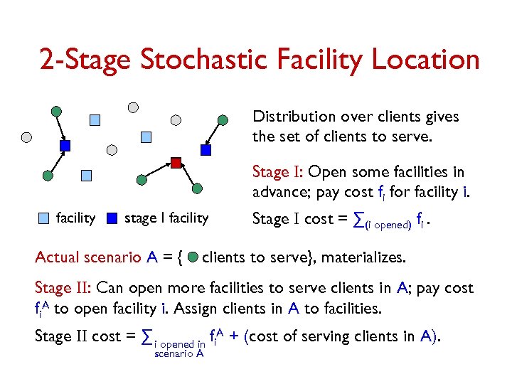
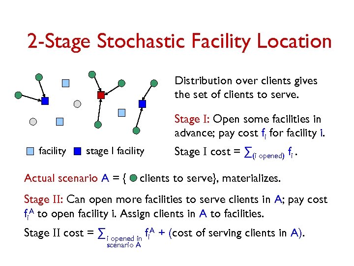2 -Stage Stochastic Facility Location Distribution over clients gives the set of clients to serve. Stage I: Open some facilities in advance; pay cost fi for facility i. facility stage I facility Actual scenario A = { Stage I cost = ∑(i opened) fi. clients to serve}, materializes. Stage II: Can open more facilities to serve clients in A; pay cost fi. A to open facility i. Assign clients in A to facilities. Stage II cost = ∑ i opened in fi. A + (cost of serving clients in A). scenario A

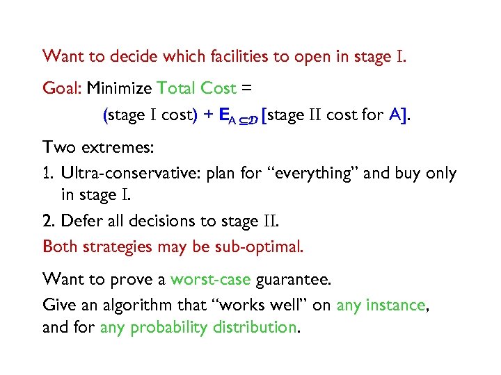Want to decide which facilities to open in stage I. Goal: Minimize Total Cost = (stage I cost) + EA ÍD [stage II cost for A]. Two extremes: 1. Ultra-conservative: plan for “everything” and buy only in stage I. 2. Defer all decisions to stage II. Both strategies may be sub-optimal. Want to prove a worst-case guarantee. Give an algorithm that “works well” on any instance, and for any probability distribution.

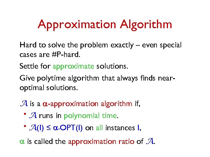Approximation Algorithm Hard to solve the problem exactly – even special cases are #P-hard. Settle for approximate solutions. Give polytime algorithm that always finds nearoptimal solutions. A is a a-approximation algorithm if, A runs in polynomial time. A(I) ≤ a. OPT(I) on all instances I, • • a is called the approximation ratio of A.

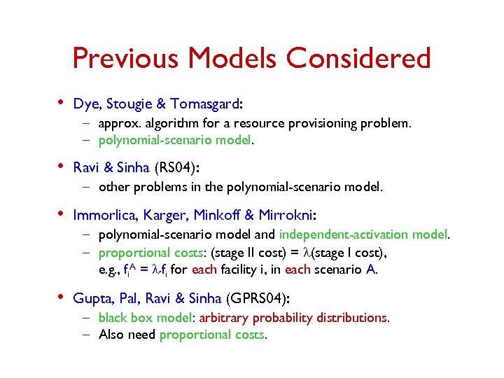Previous Models Considered • Dye, Stougie & Tomasgard: – approx. algorithm for a resource provisioning problem. – polynomial-scenario model. • Ravi & Sinha (RS 04): – other problems in the polynomial-scenario model. • Immorlica, Karger, Minkoff & Mirrokni: – polynomial-scenario model and independent-activation model. – proportional costs: (stage II cost) = l(stage I cost), e. g. , fi. A = l. fi for each facility i, in each scenario A. • Gupta, Pal, Ravi & Sinha (GPRS 04): – black box model: arbitrary probability distributions. – Also need proportional costs.

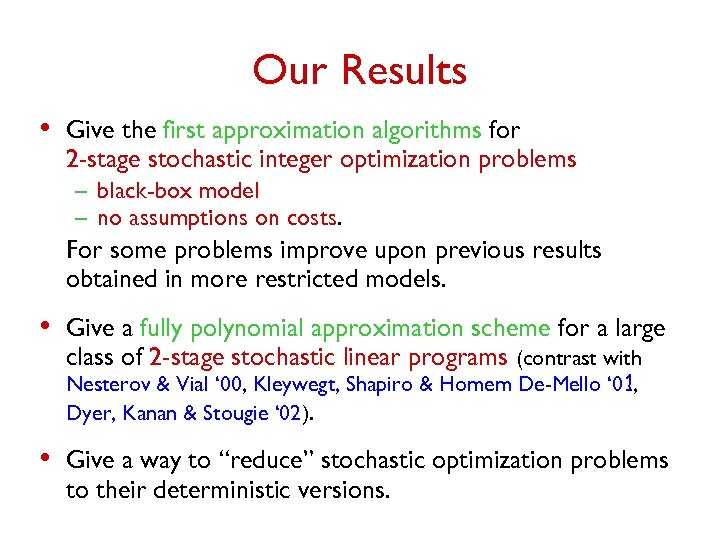Our Results • Give the first approximation algorithms for 2 -stage stochastic integer optimization problems – black-box model – no assumptions on costs. For some problems improve upon previous results obtained in more restricted models. • Give a fully polynomial approximation scheme for a large class of 2 -stage stochastic linear programs (contrast with Nesterov & Vial ‘ 00, Kleywegt, Shapiro & Homem De-Mello ‘ 01, Dyer, Kanan & Stougie ‘ 02). • Give a way to “reduce” stochastic optimization problems to their deterministic versions.

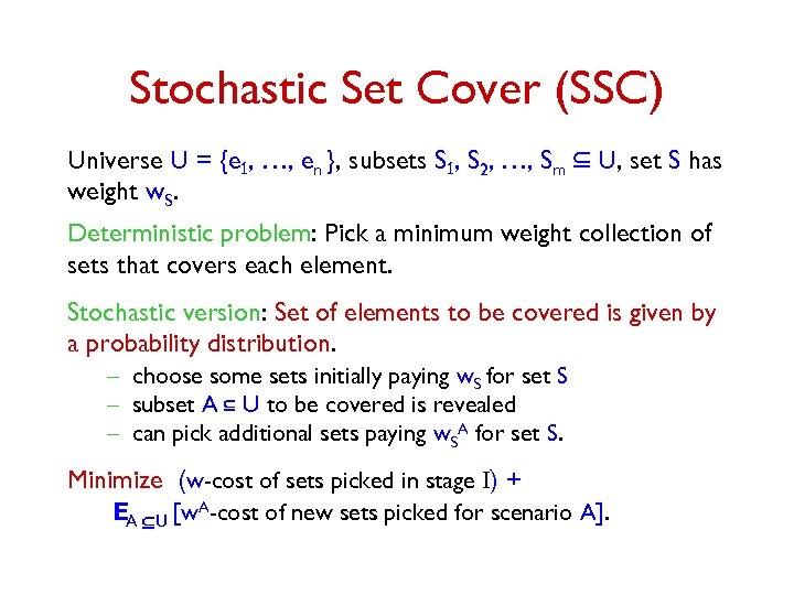Stochastic Set Cover (SSC) Universe U = {e 1, …, en }, subsets S 1, S 2, …, Sm Í U, set S has weight w. S. Deterministic problem: Pick a minimum weight collection of sets that covers each element. Stochastic version: Set of elements to be covered is given by a probability distribution. – choose some sets initially paying w. S for set S – subset A Í U to be covered is revealed – can pick additional sets paying w. SA for set S. Minimize (w-cost of sets picked in stage I) + EA ÍU [w. A-cost of new sets picked for scenario A].

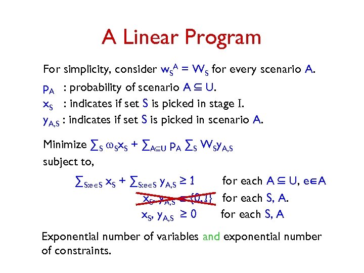A Integer Program An Linear Program For simplicity, consider w. SA = WS for every scenario A. p. A : probability of scenario A Í U. x. S : indicates if set S is picked in stage I. y. A, S : indicates if set S is picked in scenario A. Minimize ∑S w. Sx. S + ∑AÍU p. A ∑S WSy. A, S subject to, ∑S: eÎS x. S + ∑S: eÎS y. A, S ≥ 1 for each A Í U, eÎA x. S, y. A, S Î {0, 1} for each S, A. x. S, y. A, S ≥ 0 for each S, A Exponential number of variables and exponential number of constraints.

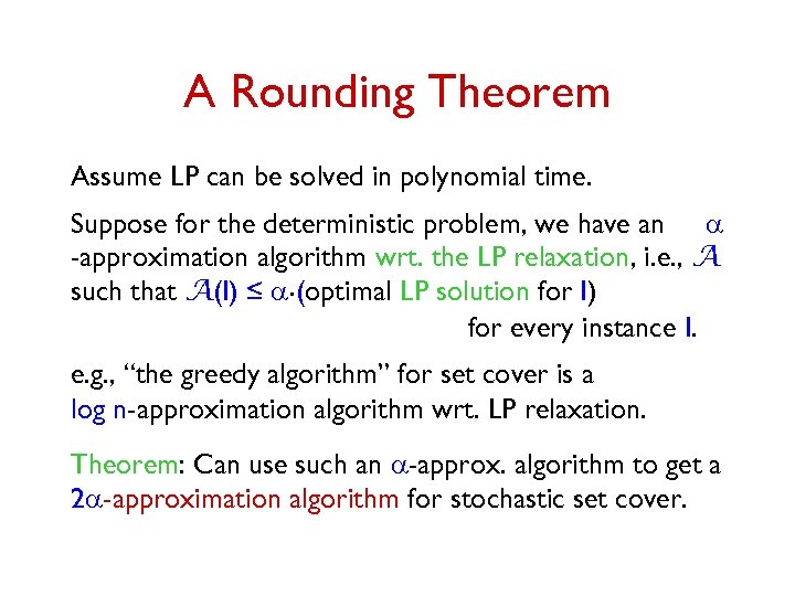A Rounding Theorem Assume LP can be solved in polynomial time. Suppose for the deterministic problem, we have an a -approximation algorithm wrt. the LP relaxation, i. e. , A such that A(I) ≤ a. (optimal LP solution for I) for every instance I. e. g. , “the greedy algorithm” for set cover is a log n-approximation algorithm wrt. LP relaxation. Theorem: Can use such an a-approx. algorithm to get a 2 a-approximation algorithm for stochastic set cover.

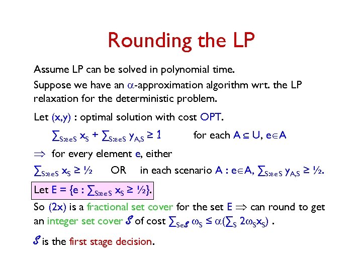
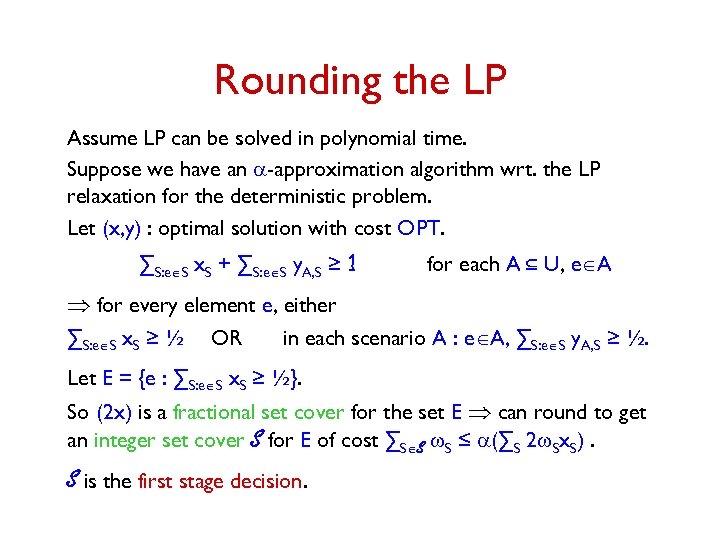Rounding the LP Assume LP can be solved in polynomial time. Suppose we have an a-approximation algorithm wrt. the LP relaxation for the deterministic problem. Let (x, y) : optimal solution with cost OPT. ∑S: eÎS x. S + ∑S: eÎS y. A, S ≥ 1 for each A Í U, eÎA Þ for every element e, either ∑S: eÎS x. S ≥ ½ OR in each scenario A : eÎA, ∑S: eÎS y. A, S ≥ ½. Let E = {e : ∑S: eÎS x. S ≥ ½}. So (2 x) is a fractional set cover for the set E Þ can round to get an integer set cover S for E of cost ∑SÎS w. S ≤ a(∑S 2 w. Sx. S). S is the first stage decision.

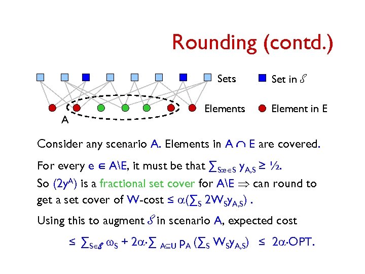Rounding (contd. ) Sets Elements A Set in S Element in E Consider any scenario A. Elements in A Ç E are covered. For every e Î AE, it must be that ∑S: eÎS y. A, S ≥ ½. So (2 y. A) is a fractional set cover for AE Þ can round to get a set cover of W-cost ≤ a(∑S 2 WSy. A, S). Using this to augment S in scenario A, expected cost ≤ ∑SÎS w. S + 2 a. ∑ AÍU p. A (∑S WSy. A, S) ≤ 2 a. OPT.

Rounding (contd. ) An a-approx. algorithm for deterministic problem gives a 2 a-approximation guarantee for stochastic problem. In the polynomial-scenario model, gives simple polytime approximation algorithms for covering problems. • 2 log n-approximation for SSC. • 4 -approximation for stochastic vertex cover. • 4 -approximation for stochastic multicut on trees. Ravi & Sinha gave a log n-approximation algorithm for SSC, 2 -approximation algorithm for stochastic vertex cover in the polynomial-scenario model.

Rounding the LP Assume LP can be solved in polynomial time. Suppose we have an a-approximation algorithm wrt. the LP relaxation for the deterministic problem. Let (x, y) : optimal solution with cost OPT. ∑S: eÎS x. S + ∑S: eÎS y. A, S ≥ 1 for each A Í U, eÎA Þ for every element e, either ∑S: eÎS x. S ≥ ½ OR in each scenario A : eÎA, ∑S: eÎS y. A, S ≥ ½. Let E = {e : ∑S: eÎS x. S ≥ ½}. So (2 x) is a fractional set cover for the set E Þ can round to get an integer set cover S of cost ∑SÎS w. S ≤ a(∑S 2 w. Sx. S). S is the first stage decision.

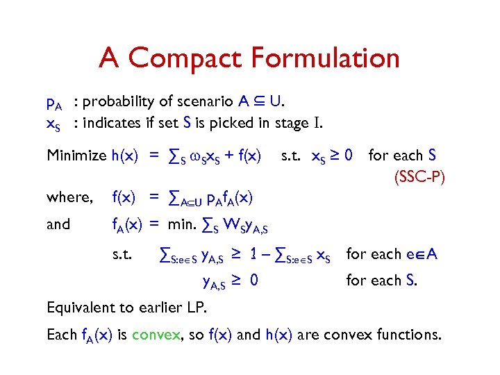A Compact Formulation p. A : probability of scenario A Í U. x. S : indicates if set S is picked in stage I. Minimize h(x) = ∑S w. Sx. S + f(x) where, f(x) = ∑AÍU p. Af. A(x) and s. t. x. S ≥ 0 for each S (SSC-P) f. A(x) = min. ∑S WSy. A, S s. t. ∑S: eÎS y. A, S ≥ 1 – ∑S: eÎS x. S for each eÎA y. A, S ≥ 0 for each S. Equivalent to earlier LP. Each f. A(x) is convex, so f(x) and h(x) are convex functions.

The General Strategy 1. Get a (1+e)-optimal solution (x) to the convex program using the ellipsoid method. 2. Convert fractional solution (x) to integer solution – decouple stage I and stage II scenarios – use a-approx. algorithm for the deterministic problem to solve subproblems. Obtain a c. a-approximation algorithm for the stochastic integer problem.

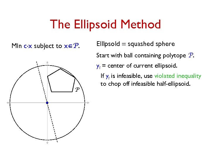The Ellipsoid Method Min c. x subject to xÎP. Ellipsoid º squashed sphere Start with ball containing polytope P. yi = center of current ellipsoid. P If yi is infeasible, use violated inequality to chop off infeasible half-ellipsoid.

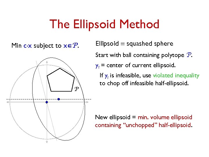The Ellipsoid Method Min c. x subject to xÎP. Ellipsoid º squashed sphere Start with ball containing polytope P. yi = center of current ellipsoid. P If yi is infeasible, use violated inequality to chop off infeasible half-ellipsoid. New ellipsoid = min. volume ellipsoid containing “unchopped” half-ellipsoid.

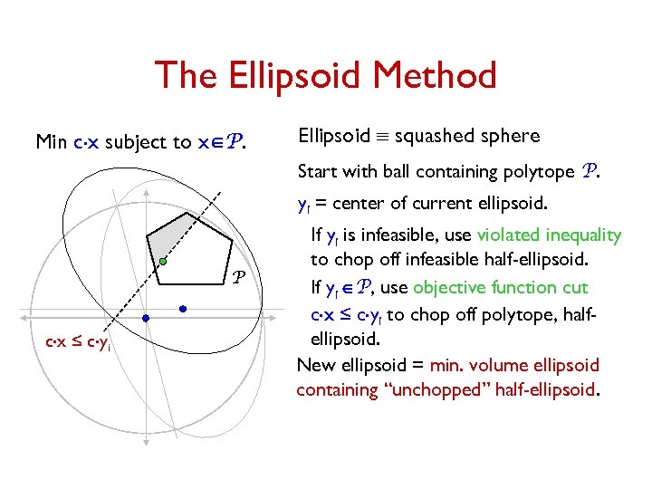The Ellipsoid Method Min c. x subject to xÎP. Ellipsoid º squashed sphere Start with ball containing polytope P. yi = center of current ellipsoid. P c. x ≤ c. y i If yi is infeasible, use violated inequality to chop off infeasible half-ellipsoid. If yi ÎP, use objective function cut c. x ≤ c. yi to chop off polytope, halfellipsoid. New ellipsoid = min. volume ellipsoid containing “unchopped” half-ellipsoid.

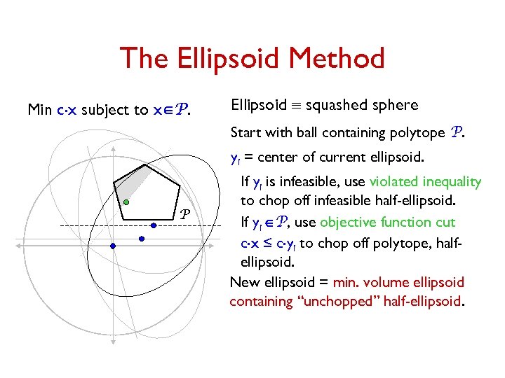The Ellipsoid Method Min c. x subject to xÎP. Ellipsoid º squashed sphere Start with ball containing polytope P. yi = center of current ellipsoid. P If yi is infeasible, use violated inequality to chop off infeasible half-ellipsoid. If yi ÎP, use objective function cut c. x ≤ c. yi to chop off polytope, halfellipsoid. New ellipsoid = min. volume ellipsoid containing “unchopped” half-ellipsoid.

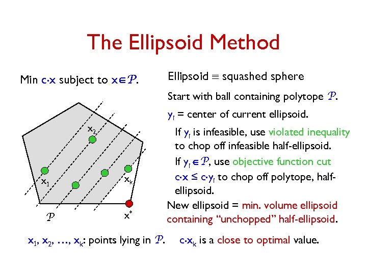The Ellipsoid Method Min c. x subject to xÎP. Ellipsoid º squashed sphere Start with ball containing polytope P. yi = center of current ellipsoid. x 2 x 1 P xk x* x 1, x 2, …, xk: points lying in P. If yi is infeasible, use violated inequality to chop off infeasible half-ellipsoid. If yi ÎP, use objective function cut c. x ≤ c. yi to chop off polytope, halfellipsoid. New ellipsoid = min. volume ellipsoid containing “unchopped” half-ellipsoid. c. xk is a close to optimal value.

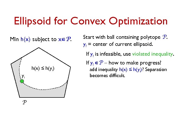Ellipsoid for Convex Optimization Min h(x) subject to xÎP. Start with ball containing polytope P. yi = center of current ellipsoid. If yi is infeasible, use violated inequality. h(x) ≤ h(yi) yi P If yi ÎP – how to make progress? add inequality h(x) ≤ h(yi)? Separation becomes difficult.

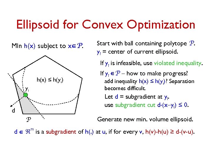Ellipsoid for Convex Optimization Min h(x) subject to xÎP. Start with ball containing polytope P. yi = center of current ellipsoid. If yi is infeasible, use violated inequality. h(x) ≤ h(yi) yi d P If yi ÎP – how to make progress? add inequality h(x) ≤ h(yi)? Separation becomes difficult. Let d = subgradient at yi. use subgradient cut d. (x–yi) ≤ 0. Generate new min. volume ellipsoid. d Î m is a subgradient of h(. ) at u, if for every v, h(v)-h(u) ≥ d. (v-u).

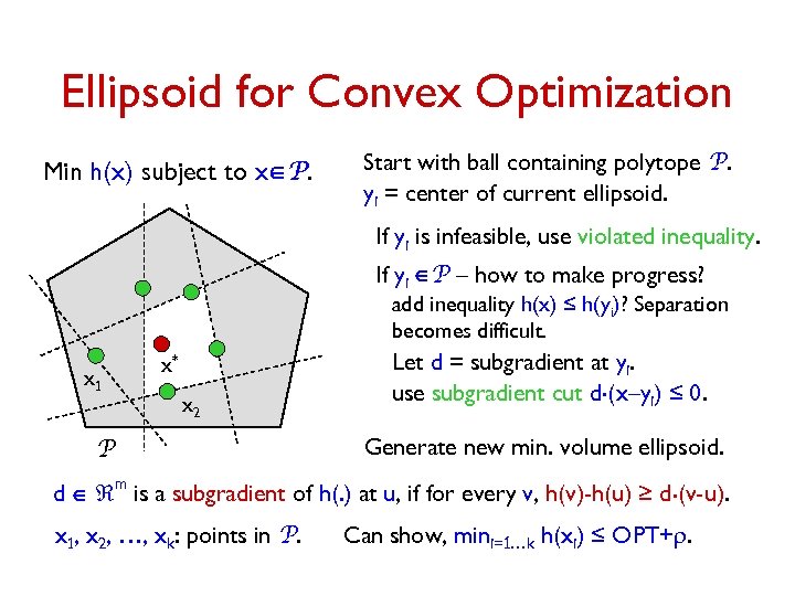Ellipsoid for Convex Optimization Min h(x) subject to xÎP. Start with ball containing polytope P. yi = center of current ellipsoid. If yi is infeasible, use violated inequality. If yi ÎP – how to make progress? add inequality h(x) ≤ h(yi)? Separation becomes difficult. x 1 x* x 2 P Let d = subgradient at yi. use subgradient cut d. (x–yi) ≤ 0. Generate new min. volume ellipsoid. d Î m is a subgradient of h(. ) at u, if for every v, h(v)-h(u) ≥ d. (v-u). x 1, x 2, …, xk: points in P. Can show, mini=1…k h(xi) ≤ OPT+r.

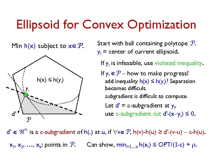Ellipsoid for Convex Optimization Min h(x) subject to xÎP. Start with ball containing polytope P. yi = center of current ellipsoid. If yi is infeasible, use violated inequality. h(x) ≤ h(yi) yi d' P If yi ÎP – how to make progress? add inequality h(x) ≤ h(yi)? Separation becomes difficult. subgradient is difficult to compute. Let d' = e-subgradient at yi. use e-subgradient cut d'. (x–yi) ≤ 0. d' Î m is a e-subgradient of h(. ) at u, if "vÎP, h(v)-h(u) ≥ d'. (v-u) – e. h(u). x 1, x 2, …, xk: points in P. Can show, mini=1…k h(xi) ≤ OPT/(1 -e) + r.

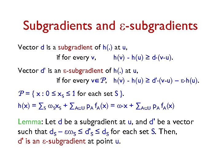Subgradients and e-subgradients Vector d is a subgradient of h(. ) at u, if for every v, h(v) - h(u) ≥ d. (v-u). Vector d' is an e-subgradient of h(. ) at u, if for every vÎP, h(v) - h(u) ≥ d'. (v-u) – e. h(u). P = { x : 0 ≤ x. S ≤ 1 for each set S }. h(x) = ∑S w. Sx. S + ∑AÍU p. A f. A(x) = w. x + ∑AÍU p. A f. A(x) Lemma: Let d be a subgradient at u, and d' be a vector such that d. S – ew. S ≤ d'S ≤ d. S for each set S. Then, d' is an e-subgradient at point u.

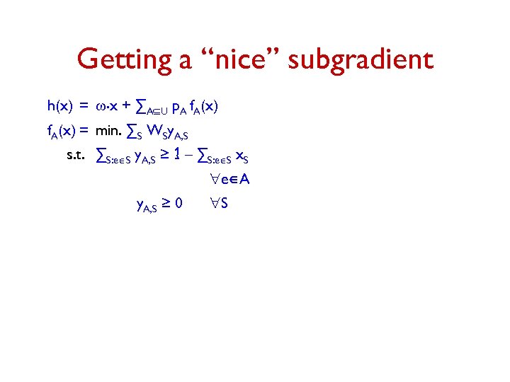Getting a “nice” subgradient h(x) = w. x + ∑AÍU p. A f. A(x) = min. ∑S WSy. A, S s. t. ∑S: eÎS y. A, S ≥ 1 – ∑S: eÎS x. S "eÎA y. A, S ≥ 0 "S

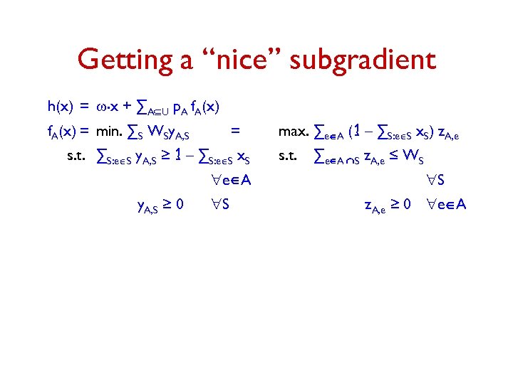Getting a “nice” subgradient h(x) = w. x + ∑AÍU p. A f. A(x) = min. ∑S WSy. A, S = s. t. ∑S: eÎS y. A, S ≥ 1 – ∑S: eÎS x. S "eÎA y. A, S ≥ 0 "S max. ∑eÎA (1 – ∑S: eÎS x. S) z. A, e s. t. ∑eÎA ÇS z. A, e ≤ WS "S z. A, e ≥ 0 "eÎA

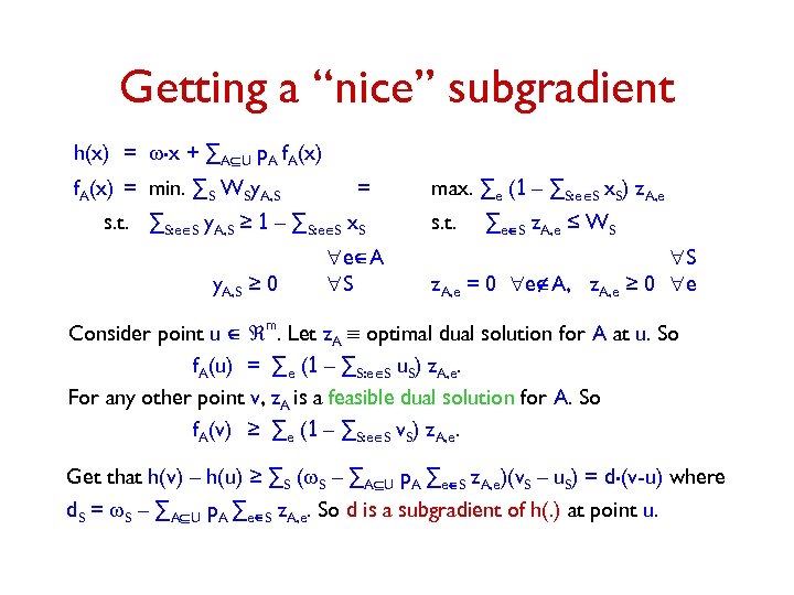Getting a “nice” subgradient h(x) = w. x + ∑AÍU p. A f. A(x) = min. ∑S WSy. A, S = s. t. ∑S: eÎS y. A, S ≥ 1 – ∑S: eÎS x. S y. A, S ≥ 0 "eÎA "S max. ∑e (1 – ∑S: eÎS x. S) z. A, e s. t. ∑eÎS z. A, e ≤ WS "S z. A, e = 0 "eÏA, z. A, e ≥ 0 "e m Consider point u Î . Let z. A º optimal dual solution for A at u. So f. A(u) = ∑e (1 – ∑S: eÎS u. S) z. A, e. For any other point v, z. A is a feasible dual solution for A. So f. A(v) ≥ ∑e (1 – ∑S: eÎS v. S) z. A, e. Get that h(v) – h(u) ≥ ∑S (w. S – ∑AÍU p. A ∑eÎS z. A, e)(v. S – u. S) = d. (v-u) where d. S = w. S – ∑AÍU p. A ∑eÎS z. A, e. So d is a subgradient of h(. ) at point u.

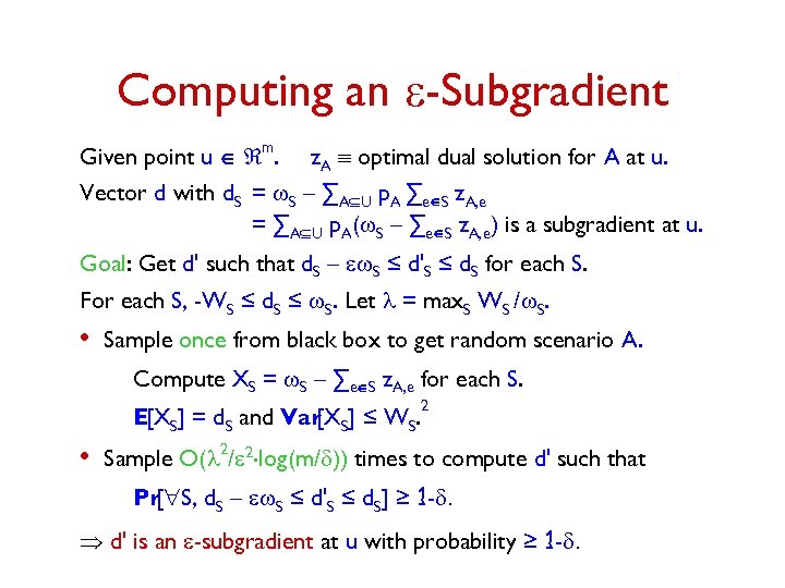Computing an e-Subgradient Given point u Î m. z. A º optimal dual solution for A at u. Vector d with d. S = w. S – ∑AÍU p. A ∑eÎS z. A, e = ∑AÍU p. A(w. S – ∑eÎS z. A, e) is a subgradient at u. Goal: Get d' such that d. S – ew. S ≤ d'S ≤ d. S for each S. For each S, -WS ≤ d. S ≤ w. S. Let l = max. S WS /w. S. • Sample once from black box to get random scenario A. Compute XS = w. S – ∑eÎS z. A, e for each S. 2 E[XS] = d. S and Var S] ≤ WS. [X • Sample O(l 2/e 2. log(m/d)) times to compute d' such that Pr["S, d. S – ew. S ≤ d'S ≤ d. S] ≥ 1 -d. Þ d' is an e-subgradient at u with probability ≥ 1 -d.

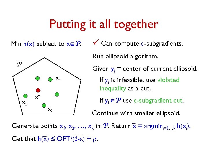Putting it all together Min h(x) subject to xÎP. ü Can compute e-subgradients. Run ellipsoid algorithm. P Given yi = center of current ellipsoid. xk x 1 If yi is infeasible, use violated inequality as a cut. x* If yi ÎP use e-subgradient cut. x 2 Continue with smaller ellipsoid. Generate points x 1, x 2, …, xk in P. Return x = argmini=1…k h(xi). Get that h(x) ≤ OPT/(1 -e) + r.

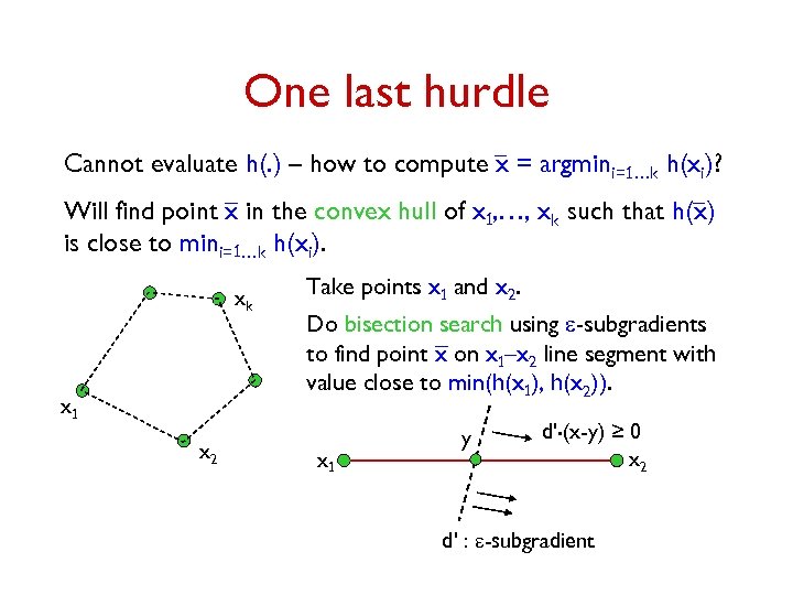One last hurdle Cannot evaluate h(. ) – how to compute x = argmini=1…k h(xi)? Will find point x in the convex hull of x 1, …, xk such that h(x) is close to mini=1…k h(xi). xk x 1 x 2 Take points x 1 and x 2. Do bisection search using e-subgradients to find point x on x 1–x 2 line segment with value close to min(h(x 1), h(x 2)). x 1 y d'. (x-y) ≥ 0 x 2 d' : e-subgradient

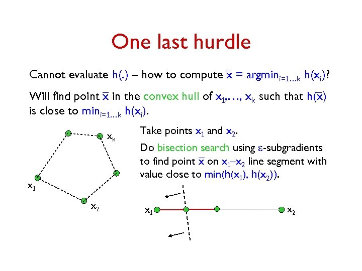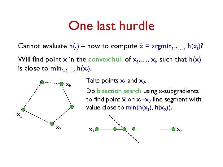One last hurdle Cannot evaluate h(. ) – how to compute x = argmini=1…k h(xi)? Will find point x in the convex hull of x 1, …, xk such that h(x) is close to mini=1…k h(xi). xk x 1 x 2 Take points x 1 and x 2. Do bisection search using e-subgradients to find point x on x 1–x 2 line segment with value close to min(h(x 1), h(x 2)). x 1 x 2

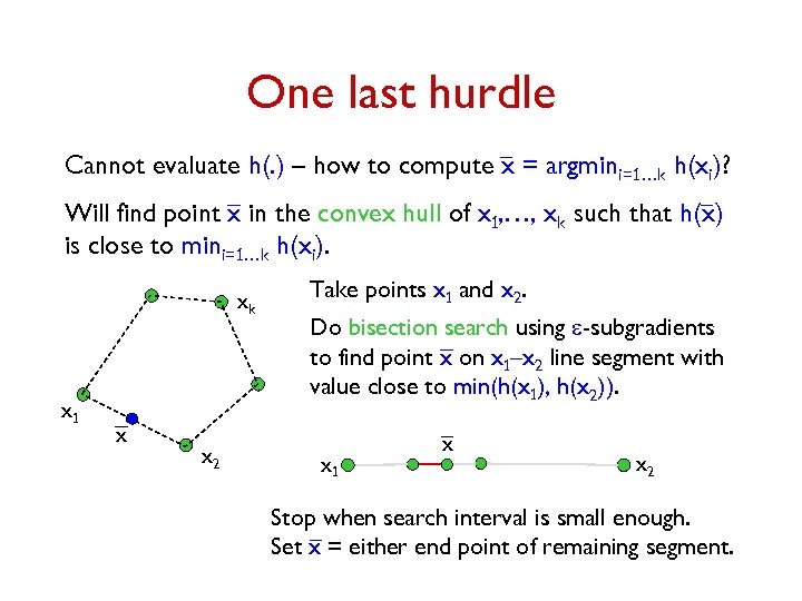One last hurdle Cannot evaluate h(. ) – how to compute x = argmini=1…k h(xi)? Will find point x in the convex hull of x 1, …, xk such that h(x) is close to mini=1…k h(xi). xk x 1 x x 2 Take points x 1 and x 2. Do bisection search using e-subgradients to find point x on x 1–x 2 line segment with value close to min(h(x 1), h(x 2)). x 1 x x 2 Stop when search interval is small enough. Set x = either end point of remaining segment.

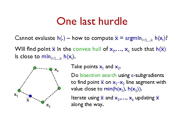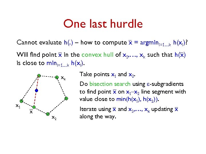One last hurdle Cannot evaluate h(. ) – how to compute x = argmini=1…k h(xi)? Will find point x in the convex hull of x 1, …, xk such that h(x) is close to mini=1…k h(xi). xk x 1 x x 2 Take points x 1 and x 2. Do bisection search using e-subgradients to find point x on x 1–x 2 line segment with value close to min(h(x 1), h(x 2)). Iterate using x and x 3, …, xk updating x along the way.

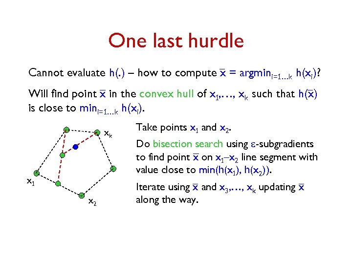One last hurdle Cannot evaluate h(. ) – how to compute x = argmini=1…k h(xi)? Will find point x in the convex hull of x 1, …, xk such that h(x) is close to mini=1…k h(xi). xk x 1 x 2 Take points x 1 and x 2. Do bisection search using e-subgradients to find point x on x 1–x 2 line segment with value close to min(h(x 1), h(x 2)). Iterate using x and x 3, …, xk updating x along the way.

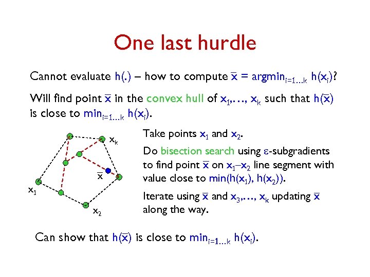One last hurdle Cannot evaluate h(. ) – how to compute x = argmini=1…k h(xi)? Will find point x in the convex hull of x 1, …, xk such that h(x) is close to mini=1…k h(xi). xk x x 1 x 2 Take points x 1 and x 2. Do bisection search using e-subgradients to find point x on x 1–x 2 line segment with value close to min(h(x 1), h(x 2)). Iterate using x and x 3, …, xk updating x along the way. Can show that h(x) is close to mini=1…k h(xi).

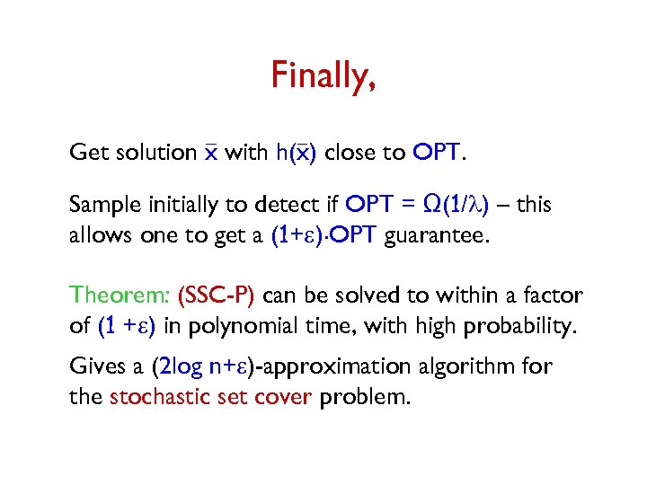Finally, Get solution x with h(x) close to OPT. Sample initially to detect if OPT = Ω(1/l) – this allows one to get a (1+e). OPT guarantee. Theorem: (SSC-P) can be solved to within a factor of (1 +e) in polynomial time, with high probability. Gives a (2 log n+e)-approximation algorithm for the stochastic set cover problem.

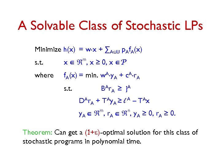A Solvable Class of Stochastic LPs Minimize h(x) = w. x + ∑AÍU p. Af. A(x) s. t. x Î m, x ≥ 0, x ÎP where f. A(x) = min. w. A. y. A + c. A. r. A s. t. B A r A ≥ j. A DAr. A + TAy. A ≥ l A – TAx y. A Î m, r. A Î n, y. A ≥ 0, r. A ≥ 0. Theorem: Can get a (1+e)-optimal solution for this class of stochastic programs in polynomial time.

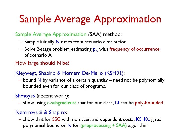Sample Average Approximation (SAA) method: – Sample initially N times from scenario distribution – Solve 2 -stage problem estimating p. A with frequency of occurrence of scenario A How large should N be? Kleywegt, Shapiro & Homem De-Mello (KSH 01): – bound N by variance of a certain quantity – need not be polynomially bounded even for our class of programs. Shmoys. S (recent work): – show using e-subgradients that for our class, N can be poly-bounded. Nemirovskii & Shapiro: – show that for SSC with non-scenario dependent costs, KSH 01 gives polynomial bound on N for (preprocessing + SAA) algorithm.

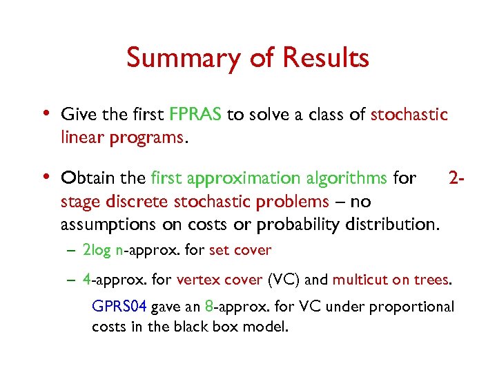Summary of Results • Give the first FPRAS to solve a class of stochastic linear programs. • Obtain the first approximation algorithms for 2 - stage discrete stochastic problems – no assumptions on costs or probability distribution. – 2 log n-approx. for set cover – 4 -approx. for vertex cover (VC) and multicut on trees. GPRS 04 gave an 8 -approx. for VC under proportional costs in the black box model.

Results (contd. ) – 3. 23 -approx. for uncapacitated facility location (FL). Get constant guarantees for several variants such as FL with penalties, or soft capacities, or services. Improve upon results of GPRS 04, RS 04 obtained in restricted models. – (1+e)-approx. for multicommodity flow. Immorlica et al. gave optimal algorithm for singlecommodity in polynomial “scenario” (demand) case. • Give a general technique to lift deterministic guarantees to stochastic setting.

Open Questions • Practical Impact: Can one use e-subgradients in other deterministic optimization methods, e. g. , cutting plane methods? Interior-point algorithms? • Multi-stage stochastic optimization. • Characterize which deterministic problems are “easy to solve” in stochastic setting, and which problems are “hard”.

Thank You.