Stochastic Optimization ESI 6912 NOTES 7 Algorithms and

Stochastic Optimization ESI 6912 NOTES 7: Algorithms and Applications Instructor: Prof. S. Uryasev

Content 1. Value-at-Risk (Va. R) a. Definition b. Features c. Examples 2. Conditional Value-at-Risk (CVa. R) a. Definition: Continuous and Discrete distribution b. Features c. Examples 3. Formulation of optimization problem a. Definition of a loss function b. Examples: CVa. R in performance function and CVa. R in constraints 4. Optimization techniques a. CVa. R as an optimization problem: Theorem 1 and Theorem 2 b. Reduction to LP 5. Case Studies

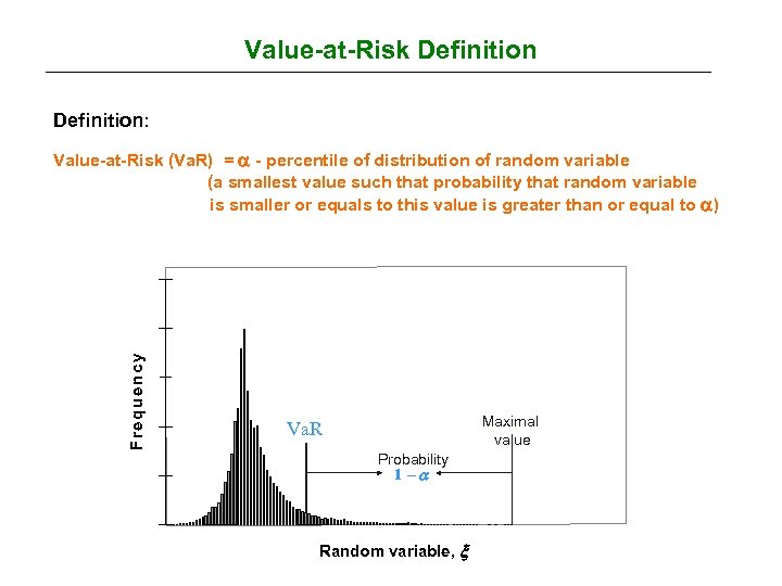Value-at-Risk Definition: F re q u e n c y Value-at-Risk (Va. R) = - percentile of distribution of random variable (a smallest value such that probability that random variable is smaller or equals to this value is greater than or equal to ) Maximal value Va. R Probability 1 - Random variable,

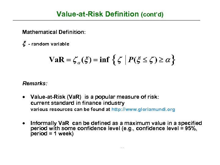Value-at-Risk Definition (cont’d) Mathematical Definition: - random variable Remarks: · Value-at-Risk (Va. R) is a popular measure of risk: current standard in finance industry various resources can be found at http: //www. gloriamundi. org · Informally Va. R can be defined as a maximum value in a specified period with some confidence level (e. g. , confidence level = 95%, period = 1 week)

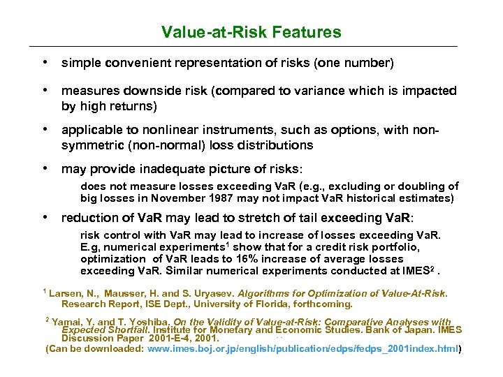Value-at-Risk Features • simple convenient representation of risks (one number) • measures downside risk (compared to variance which is impacted by high returns) • applicable to nonlinear instruments, such as options, with nonsymmetric (non-normal) loss distributions • may provide inadequate picture of risks: does not measure losses exceeding Va. R (e. g. , excluding or doubling of big losses in November 1987 may not impact Va. R historical estimates) • reduction of Va. R may lead to stretch of tail exceeding Va. R: risk control with Va. R may lead to increase of losses exceeding Va. R. E. g, numerical experiments 1 show that for a credit risk portfolio, optimization of Va. R leads to 16% increase of average losses exceeding Va. R. Similar numerical experiments conducted at IMES 2. 1 Larsen, N. , Mausser, H. and S. Uryasev. Algorithms for Optimization of Value-At-Risk. Research Report, ISE Dept. , University of Florida, forthcoming. Yamai, Y. and T. Yoshiba. On the Validity of Value-at-Risk: Comparative Analyses with Expected Shortfall. Institute for Monetary and Economic Studies. Bank of Japan. IMES Discussion Paper 2001 -E-4, 2001. (Can be downloaded: www. imes. boj. or. jp/english/publication/edps/fedps_2001 index. html) 2

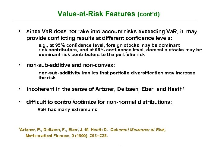Value-at-Risk Features (cont’d) • since Va. R does not take into account risks exceeding Va. R, it may provide conflicting results at different confidence levels: e. g. , at 95% confidence level, foreign stocks may be dominant risk contributors, and at 99% confidence level, domestic stocks may be dominant risk contributors to the portfolio risk • non-sub-additive and non-convex: non-sub-additivity implies that portfolio diversification may increase the risk • incoherent in the sense of Artzner, Delbaen, Eber, and Heath 1 • difficult to control/optimize for non-normal distributions: Va. R has many extremums 1 Artzner, P. , Delbaen, F. , Eber, J. -M. Heath D. Coherent Measures of Risk, Mathematical Finance, 9 (1999), 203 --228.

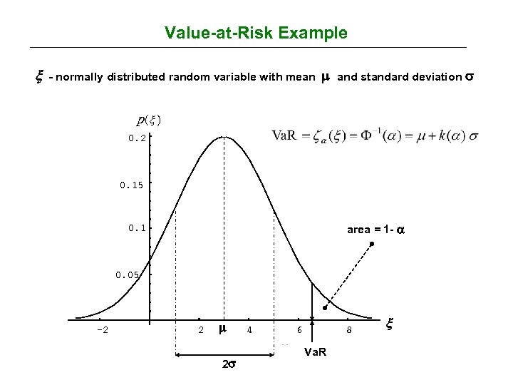Value-at-Risk Example - normally distributed random variable with mean and standard deviation p( ) 0. 2 0. 15 area = 1 - 0. 1 0. 05 -2 2 2 4 6 8 Va. R

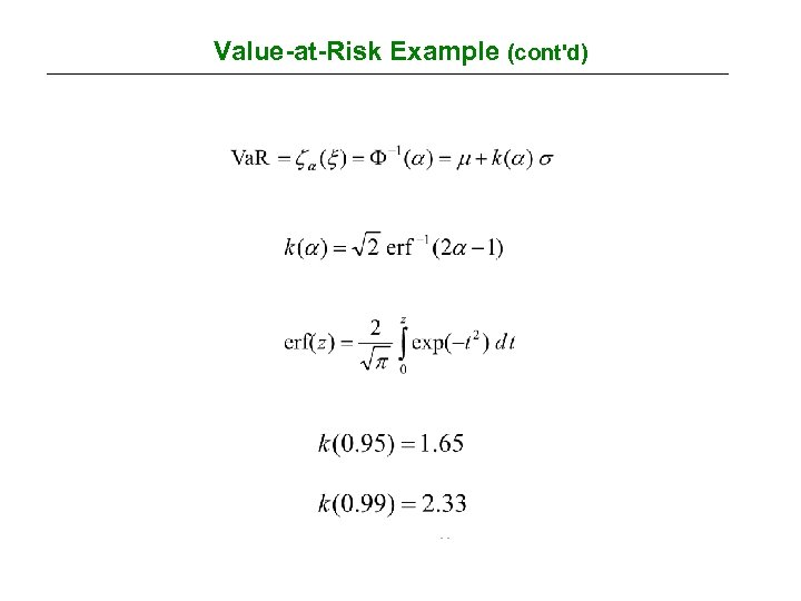Value-at-Risk Example (cont'd)

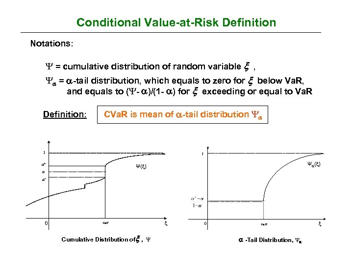Conditional Value-at-Risk Definition Notations: Ψ = cumulative distribution of random variable , Ψ = -tail distribution, which equals to zero for below Va. R, and equals to (Ψ- )/(1 - ) for exceeding or equal to Va. R Definition: CVa. R is mean of -tail distribution Ψ 1 1 a+ Ψ ( ) Ψ( ) a a- 0 Va. R Cumulative Distribution of , Ψ 0 Va. R -Tail Distribution, Ψ

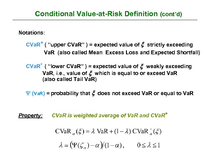Conditional Value-at-Risk Definition (cont’d) Notations: CVa. R+ ( “upper CVa. R” ) = expected value of strictly exceeding Va. R (also called Mean Excess Loss and Expected Shortfall) CVa. R- ( “lower CVa. R” ) = expected value of weakly exceeding Va. R, i. e. , value of which is equal to or exceed Va. R (also called Tail Va. R) Ψ (Va. R) = probability that does not exceed Va. R or equal to Va. R Property: CVa. R is weighted average of Va. R and CVa. R+

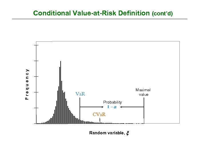F re q u e n cy Conditional Value-at-Risk Definition (cont’d) Maximal value Va. R Probability 1 - CVa. R Random variable,

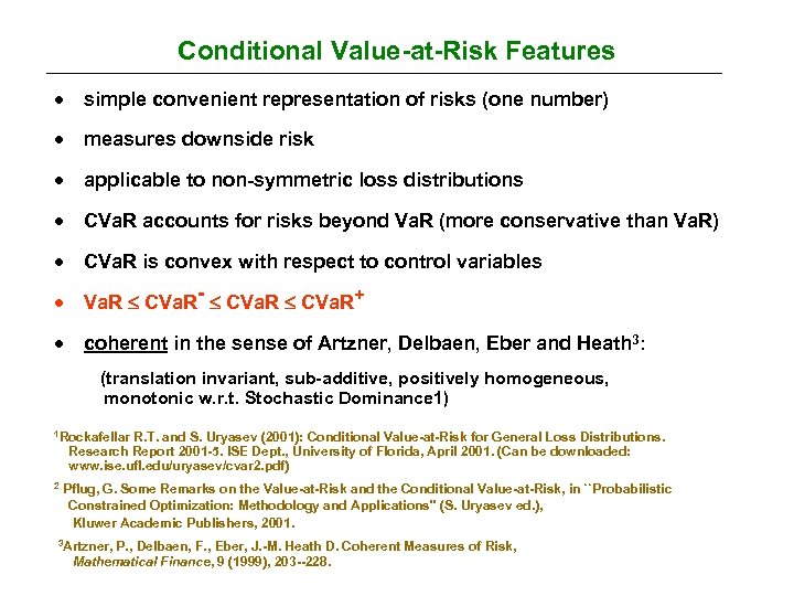Conditional Value-at-Risk Features · simple convenient representation of risks (one number) · measures downside risk · applicable to non-symmetric loss distributions · CVa. R accounts for risks beyond Va. R (more conservative than Va. R) · CVa. R is convex with respect to control variables · Va. R CVa. R- CVa. R+ · coherent in the sense of Artzner, Delbaen, Eber and Heath 3: (translation invariant, sub-additive, positively homogeneous, monotonic w. r. t. Stochastic Dominance 1) 1 Rockafellar R. T. and S. Uryasev (2001): Conditional Value-at-Risk for General Loss Distributions. Research Report 2001 -5. ISE Dept. , University of Florida, April 2001. (Can be downloaded: www. ise. ufl. edu/uryasev/cvar 2. pdf) 2 Pflug, G. Some Remarks on the Value-at-Risk and the Conditional Value-at-Risk, in ``Probabilistic Constrained Optimization: Methodology and Applications'' (S. Uryasev ed. ), Kluwer Academic Publishers, 2001. 3 Artzner, P. , Delbaen, F. , Eber, J. -M. Heath D. Coherent Measures of Risk, Mathematical Finance, 9 (1999), 203 --228.

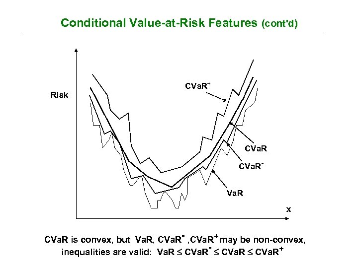Conditional Value-at-Risk Features (cont'd) Risk CVa. R+ CVa. RVa. R x CVa. R is convex, but Va. R, CVa. R- , CVa. R+ may be non-convex, inequalities are valid: Va. R CVa. R- CVa. R+

Conditional Value-at-Risk Features (cont'd) · stable statistical estimates (CVa. R has integral characteristics compared to Va. R which may be significantly impacted by one scenario) · CVa. R is continuous with respect to confidence level , consistent at different confidence levels compared to Va. R ( Va. R, CVa. R-, CVa. R+ may be discontinuous in ) · consistency with mean-variance approach: for normal loss distributions optimal variance and CVa. R portfolios coincide · easy to control/optimize for non-normal distributions; linear programming (LP): can be used for optimization of very large problems (over 1, 000 instruments and scenarios); fast, stable algorithms · loss distribution can be shaped using CVa. R constraints (many LP · can be used in fast online procedures constraints with various confidence levels in different intervals)

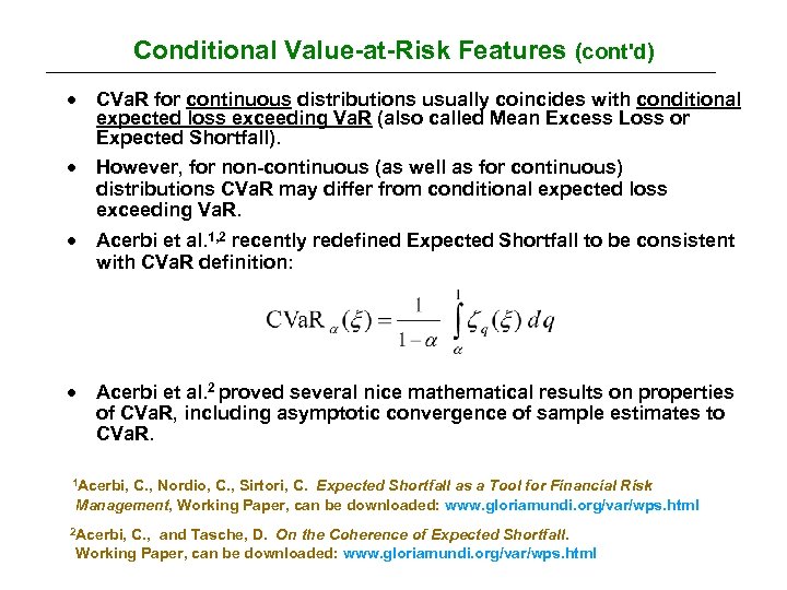Conditional Value-at-Risk Features (cont'd) · CVa. R for continuous distributions usually coincides with conditional expected loss exceeding Va. R (also called Mean Excess Loss or Expected Shortfall). · However, for non-continuous (as well as for continuous) distributions CVa. R may differ from conditional expected loss exceeding Va. R. · Acerbi et al. 1, 2 recently redefined Expected Shortfall to be consistent with CVa. R definition: · Acerbi et al. 2 proved several nice mathematical results on properties of CVa. R, including asymptotic convergence of sample estimates to CVa. R. 1 Acerbi, C. , Nordio, C. , Sirtori, C. Expected Shortfall as a Tool for Financial Risk Management, Working Paper, can be downloaded: www. gloriamundi. org/var/wps. html 2 Acerbi, C. , and Tasche, D. On the Coherence of Expected Shortfall. Working Paper, can be downloaded: www. gloriamundi. org/var/wps. html

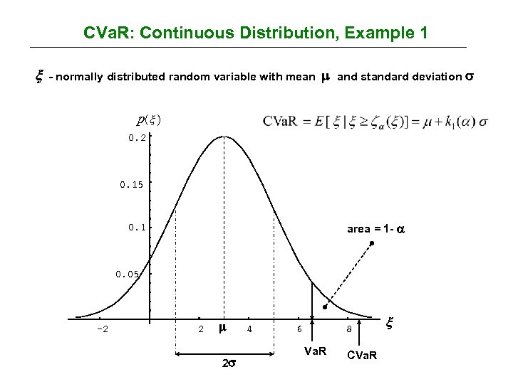CVa. R: Continuous Distribution, Example 1 - normally distributed random variable with mean and standard deviation p( ) 0. 2 0. 15 area = 1 - 0. 1 0. 05 -2 2 2 4 6 8 Va. R CVa. R

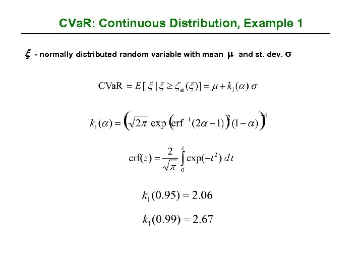CVa. R: Continuous Distribution, Example 1 - normally distributed random variable with mean and st. dev.

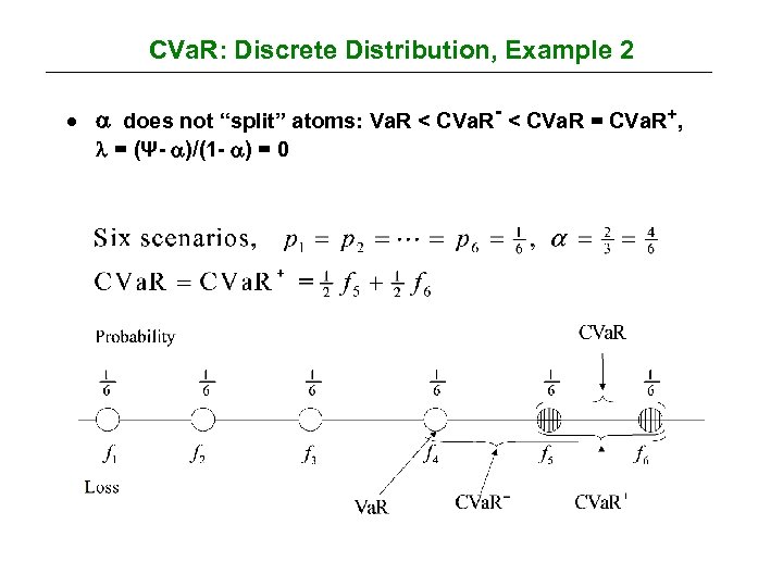CVa. R: Discrete Distribution, Example 2 · does not “split” atoms: Va. R < CVa. R- < CVa. R = CVa. R+, = (Ψ- )/(1 - ) = 0

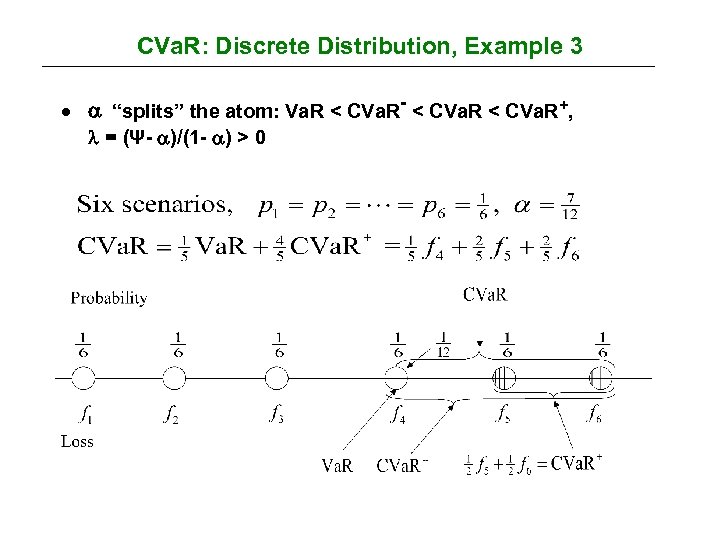CVa. R: Discrete Distribution, Example 3 · “splits” the atom: Va. R < CVa. R- < CVa. R+, = (Ψ- )/(1 - ) > 0

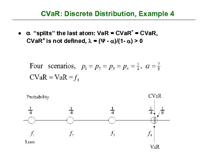CVa. R: Discrete Distribution, Example 4 · “splits” the last atom: Va. R = CVa. R- = CVa. R, CVa. R+ is not defined, = (Ψ - )/(1 - ) > 0

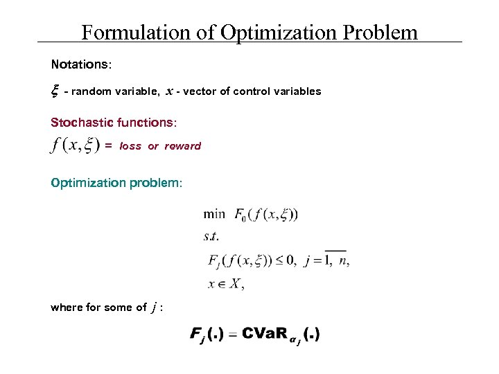Formulation of Optimization Problem Notations: - random variable, x - vector of control variables Stochastic functions: = loss or reward Optimization problem: where for some of j:

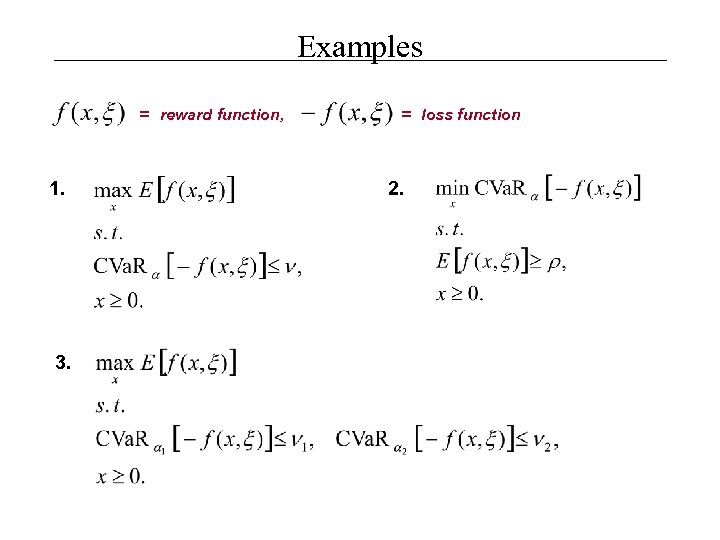Examples = reward function, 1. 3. = loss function 2.

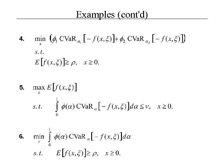Examples (cont'd) 4. 5. 6.

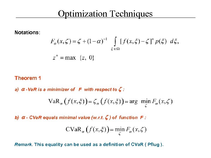Optimization Techniques Notations: Theorem 1 a) -Va. R is a minimizer of F with respect to : b) - CVa. R equals minimal value (w. r. t. ) of function F : Remark. This equality can be used as a definition of CVa. R ( Pflug ).

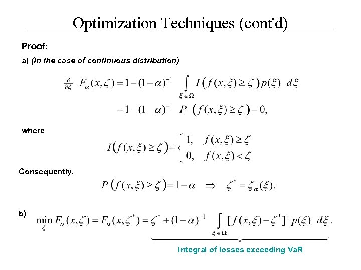Optimization Techniques (cont'd) Proof: a) (in the case of continuous distribution) where Consequently, b) Integral of losses exceeding Va. R

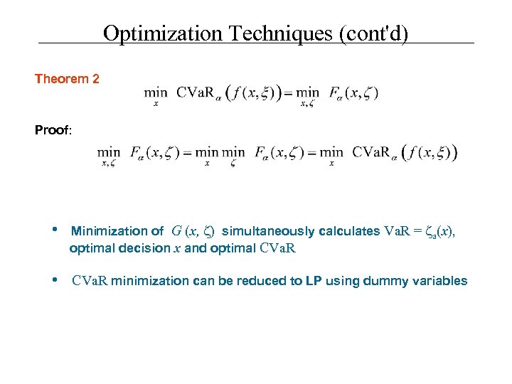Optimization Techniques (cont'd) Theorem 2 Proof: • Minimization of G (x, ) simultaneously calculates Va. R = a(x), optimal decision x and optimal CVa. R • CVa. R minimization can be reduced to LP using dummy variables

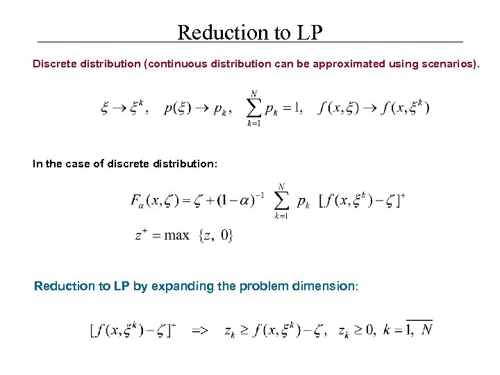Reduction to LP Discrete distribution (continuous distribution can be approximated using scenarios). In the case of discrete distribution: Reduction to LP by expanding the problem dimension:

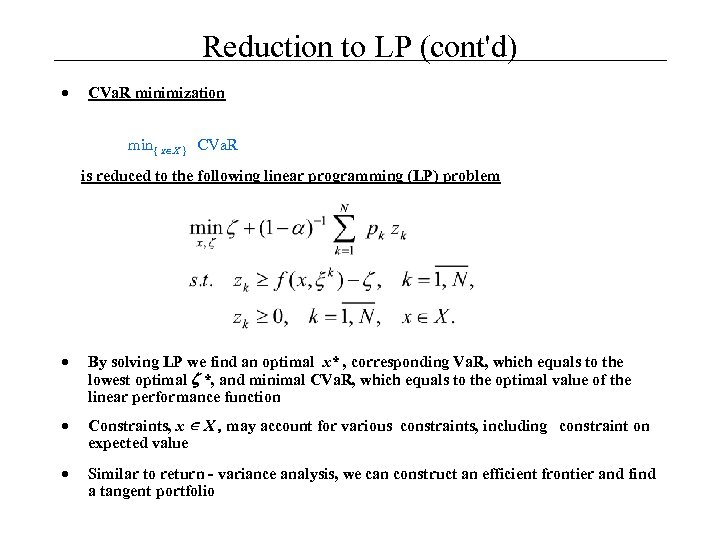Reduction to LP (cont'd) · CVa. R minimization min{ x X } CVa. R is reduced to the following linear programming (LP) problem · By solving LP we find an optimal x* , corresponding Va. R, which equals to the lowest optimal *, and minimal CVa. R, which equals to the optimal value of the linear performance function · Constraints, x X , may account for various constraints, including constraint on expected value · Similar to return - variance analysis, we can construct an efficient frontier and find a tangent portfolio

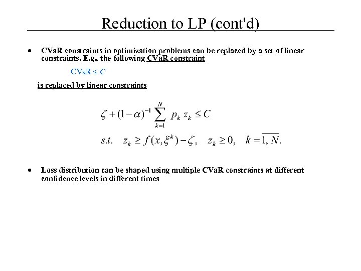Reduction to LP (cont'd) · CVa. R constraints in optimization problems can be replaced by a set of linear constraints. E. g. , the following CVa. R constraint CVa. R C is replaced by linear constraints · Loss distribution can be shaped using multiple CVa. R constraints at different confidence levels in different times

Financial Engineering Applications Portfolio optimization · Notations: x = (x 1, …, xn) = decision vector (e. g. , portfolio weights) X = a convex set of feasible decisions = ( 1, …, n) = random vector j = scenario of random vector , ( j=1, . . . J ) f(x, ) = T x = reward function - f(x, ) = - T x = loss function · Example: Two Instrument Portfolio A portfolio consists of two instruments (e. g. , options). Let x = (x 1, x 2) be a vector of positions, m = (m 1, m 2) be a vector of initial prices, and y = ( 1, 2) be a vector of uncertain prices in the next day. The loss function equals the difference between the current value of the portfolio, (x 1 m 1+x 2 m 2), and an uncertain value of the portfolio at the next day (x 1 1+x 2 2), i. e. , - f(x, ) = (x 1 m 1+x 2 m 2) – (x 1 1+x 2 2) = x 1(m 1– 1) + x 2(m 2– 2). If we do not allow short positions, the feasible set of portfolios is a two-dimensional set of non-negative numbers X = {(x 1, x 2), x 1 0, x 2 0}. Scenarios j = ( j 1, j 2), j=1, . . . J , are sample daily prices (e. g. , historical data for J trading days).

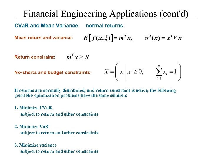Financial Engineering Applications (cont'd) CVa. R and Mean Variance: normal returns Mean return and variance: Return constraint: No-shorts and budget constraints: If returns are normally distributed, and return constraint is active, the following portfolio optimization problems have the same solution: 1. Minimize CVa. R subject to return and other constraints 2. Minimize Va. R subject to return and other constraints 3. Minimize variance subject to return and other constraints

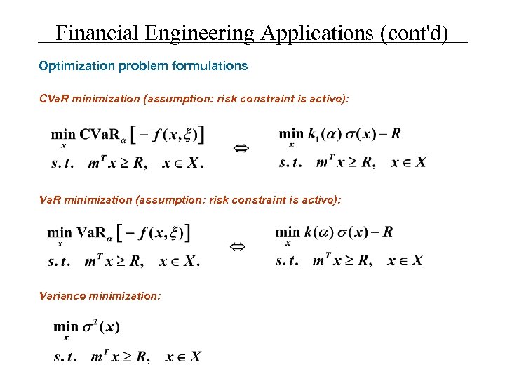Financial Engineering Applications (cont'd) Optimization problem formulations CVa. R minimization (assumption: risk constraint is active): Variance minimization:

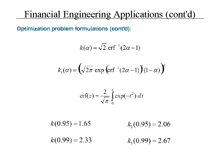Financial Engineering Applications (cont'd) Optimization problem formulations (cont'd):

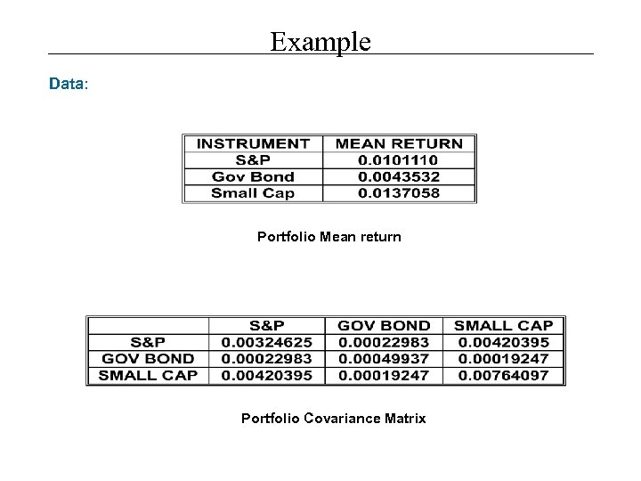Example Data: Portfolio Mean return Portfolio Covariance Matrix

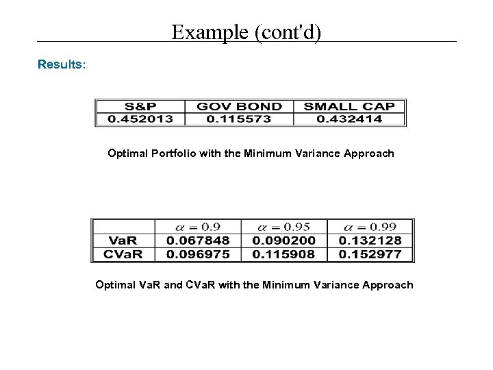Example (cont'd) Results: Optimal Portfolio with the Minimum Variance Approach Optimal Va. R and CVa. R with the Minimum Variance Approach

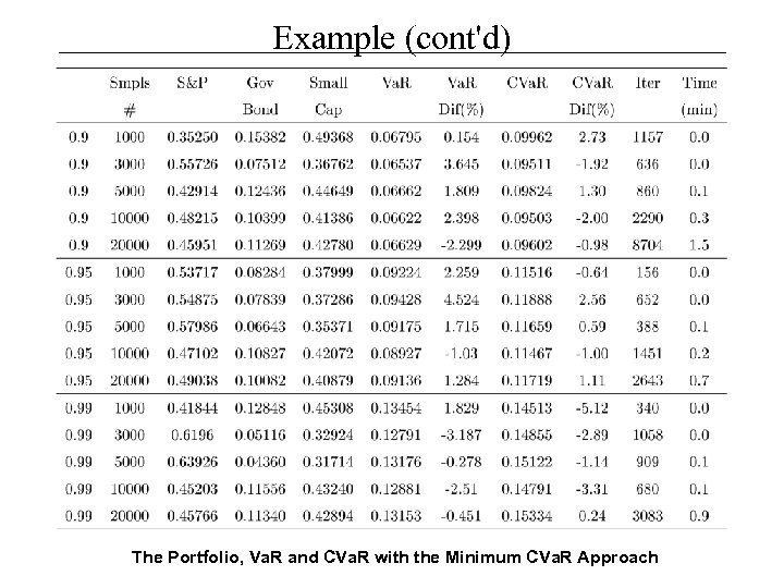Example (cont'd) The Portfolio, Va. R and CVa. R with the Minimum CVa. R Approach

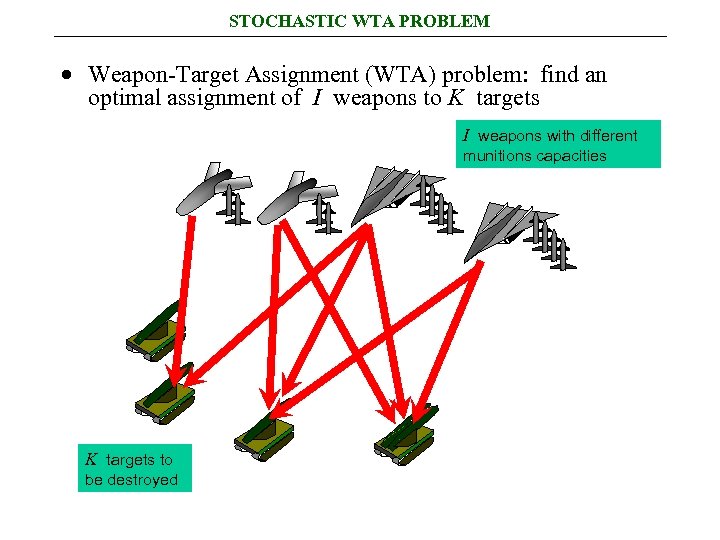STOCHASTIC WTA PROBLEM · Weapon-Target Assignment (WTA) problem: find an optimal assignment of I weapons to K targets I weapons with different munitions capacities K targets to be destroyed

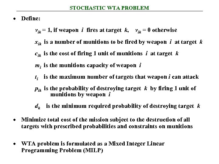STOCHASTIC WTA PROBLEM · Define: vik = 1, if weapon i fires at target k, vik = 0 otherwise xik is a number of munitions to be fired by weapon i at target k cik is the cost of firing 1 unit of munitions i at target k mi is the munitions capacity of weapon i ti is the maximum number of targets that weapon i can attack pik is the probability of destroying target k by firing 1 unit of munitions by weapon i dk is the minimum required probability of destroying target k · Minimize total cost of the mission subject to the destruction of all targets with prescribed probabilities and constraints on munitions · WTA problem is formulated as a Mixed Integer Linear Programming Problem (MILP)

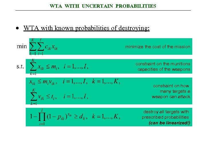WTA WITH UNCERTAIN PROBABILITIES · WTA with known probabilities of destroying: minimize the cost of the mission constraint on the munitions capacities of the weapons constraint on how many targets a weapon can attack destroy all targets with prescribed probabilities (can be linearized!)

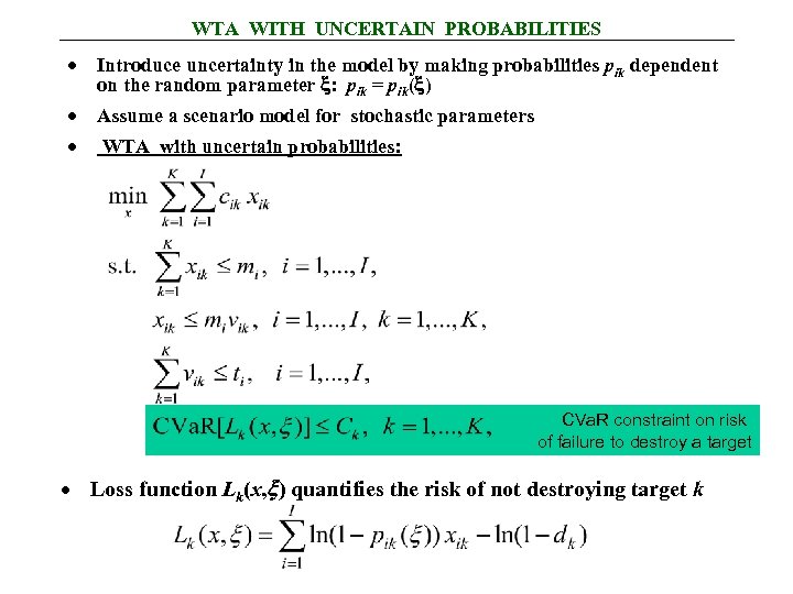WTA WITH UNCERTAIN PROBABILITIES · Introduce uncertainty in the model by making probabilities pik dependent on the random parameter : pik = pik( ) · Assume a scenario model for stochastic parameters · WTA with uncertain probabilities: CVa. R constraint on risk of failure to destroy a target · Loss function Lk(x, ) quantifies the risk of not destroying target k

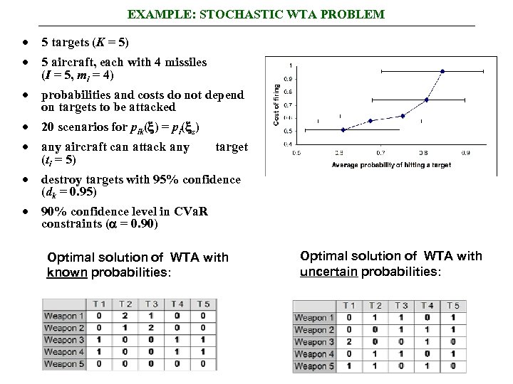EXAMPLE: STOCHASTIC WTA PROBLEM · 5 targets (K = 5) · 5 aircraft, each with 4 missiles (I = 5, mi = 4) · probabilities and costs do not depend on targets to be attacked · 20 scenarios for pik( ) = pi( s) · any aircraft can attack any target (ti = 5) · destroy targets with 95% confidence (dk = 0. 95) · 90% confidence level in CVa. R constraints ( = 0. 90) Optimal solution of WTA with known probabilities: Optimal solution of WTA with uncertain probabilities:

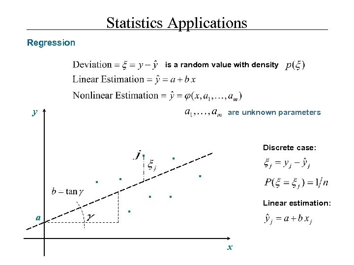Statistics Applications Regression is a random value with density y are unknown parameters . . a Discrete case: . . . Linear estimation: x

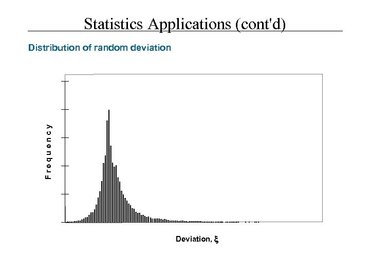Statistics Applications (cont'd) F re q u e n cy Distribution of random deviation Deviation,

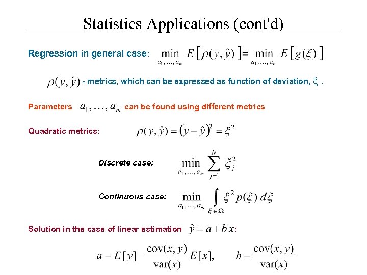Statistics Applications (cont'd) Regression in general case: - metrics, which can be expressed as function of deviation, Parameters can be found using different metrics Quadratic metrics: Discrete case: Continuous case: Solution in the case of linear estimation : .

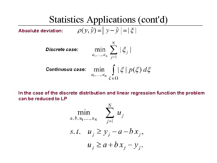Statistics Applications (cont'd) Absolute deviation: Discrete case: Continuous case: In the case of the discrete distribution and linear regression function the problem can be reduced to LP

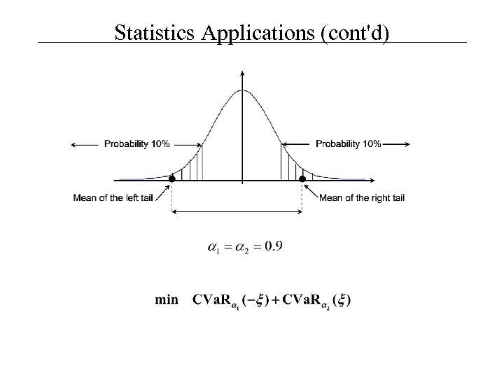Statistics Applications (cont'd)

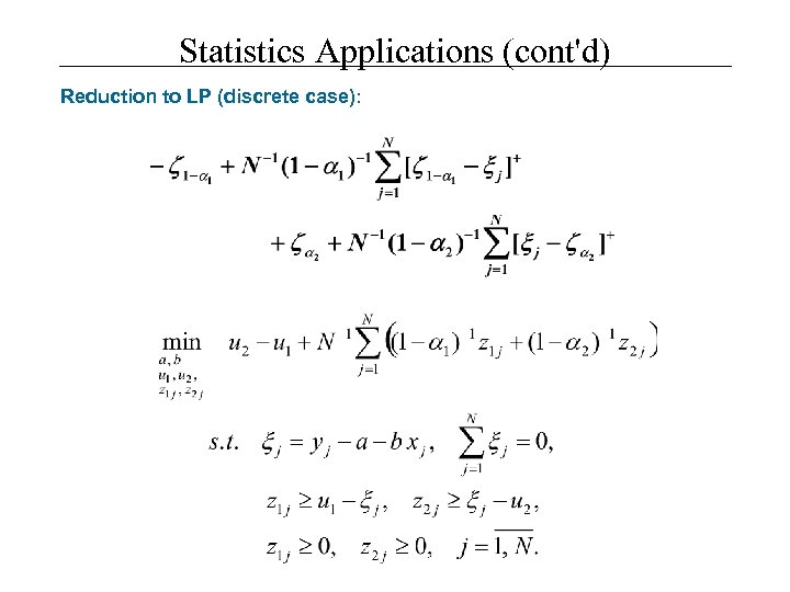Statistics Applications (cont'd) Reduction to LP (discrete case):

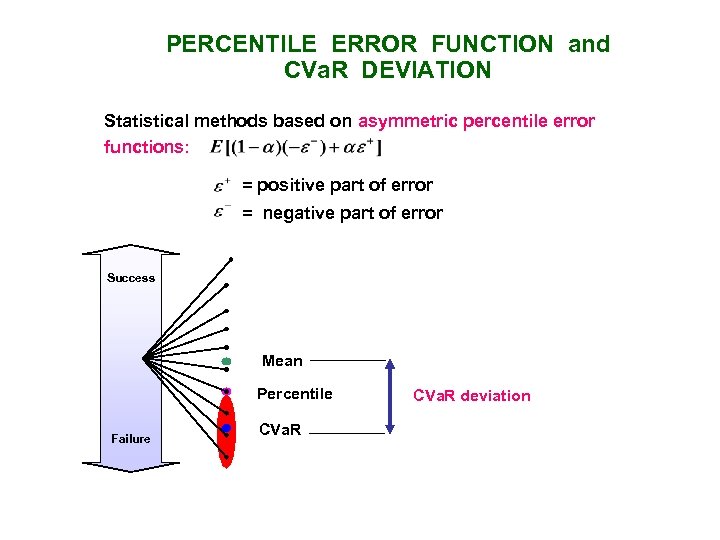
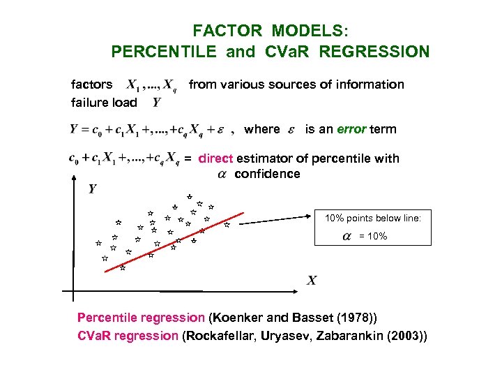FACTOR MODELS: PERCENTILE and CVa. R REGRESSION factors failure load from various sources of information where is an error term = direct estimator of percentile with confidence 10% points below line: = 10% Percentile regression (Koenker and Basset (1978)) CVa. R regression (Rockafellar, Uryasev, Zabarankin (2003))

PERCENTILE ERROR FUNCTION and CVa. R DEVIATION Statistical methods based on asymmetric percentile error functions: = positive part of error = negative part of error Success Mean Percentile Failure CVa. R deviation

Payment Deductible Premium Accident lost PDF Deductible Payment Premium Payment

PDF Deductible Premium Payment CDF 1 1 Deductible - probability of driving without accident Payment Premium Payment

Example 1: Nikkei Portfolio Distribution of losses for the NIKKEI portfolio with best normal approximation (1, 000 scenarios)

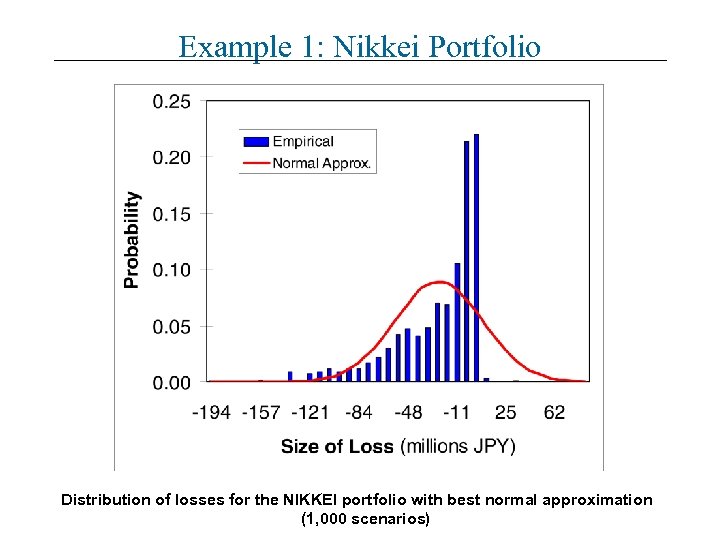
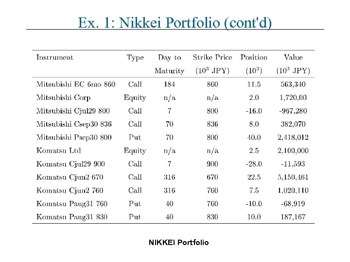Ex. 1: Nikkei Portfolio (cont'd) NIKKEI Portfolio

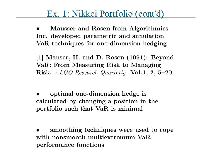Ex. 1: Nikkei Portfolio (cont'd)

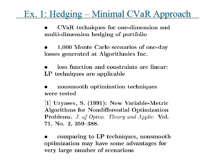Ex. 1: Hedging – Minimal CVa. R Approach

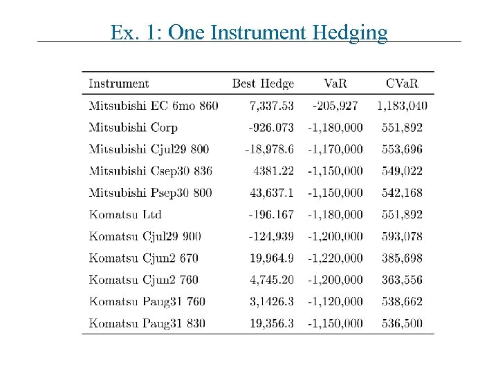Ex. 1: One Instrument Hedging

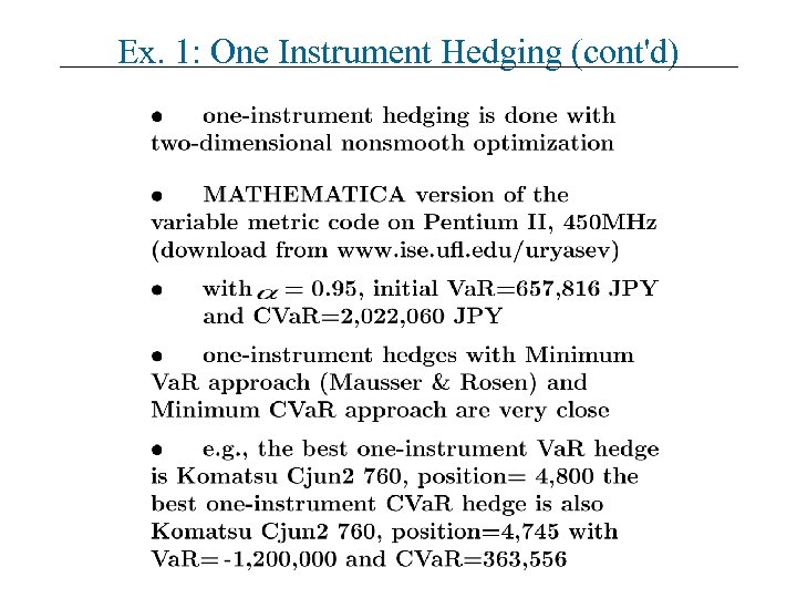Ex. 1: One Instrument Hedging (cont'd)

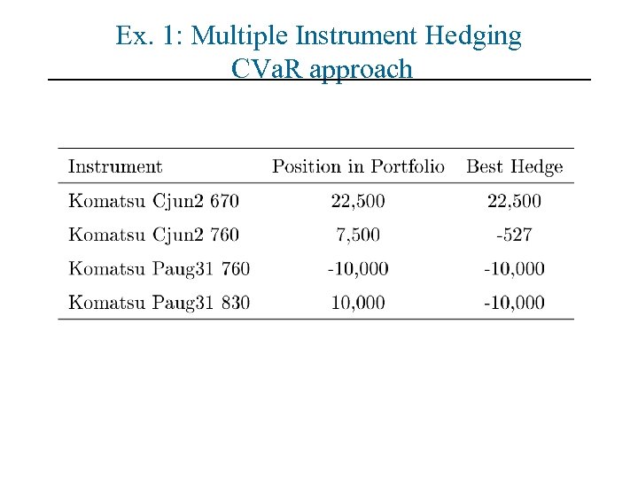Ex. 1: Multiple Instrument Hedging CVa. R approach

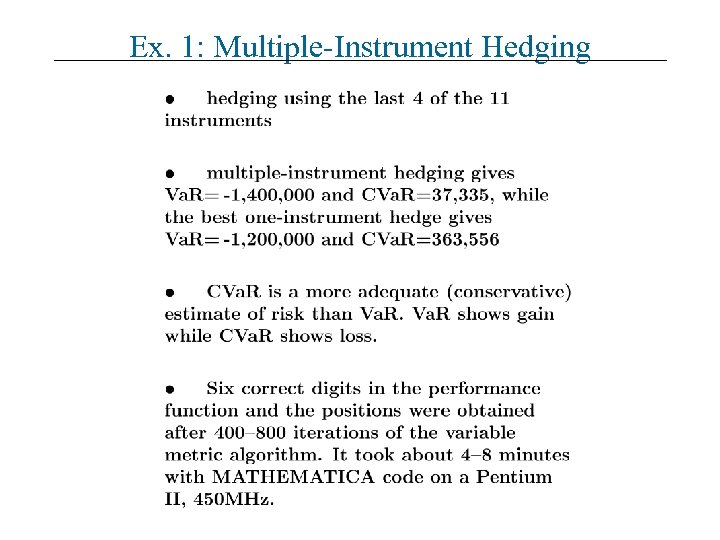Ex. 1: Multiple-Instrument Hedging

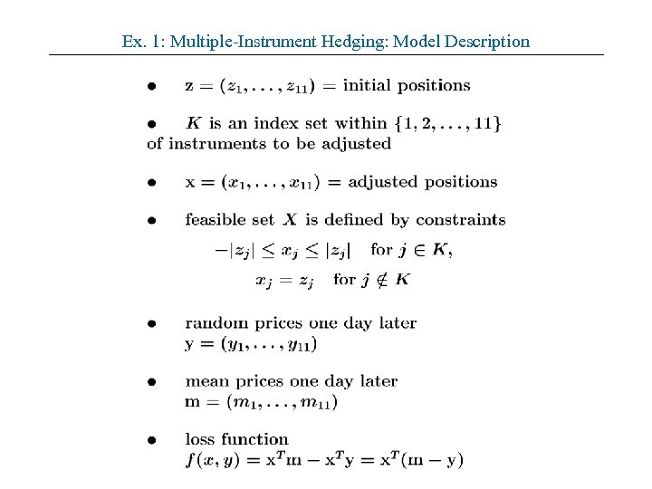Ex. 1: Multiple-Instrument Hedging: Model Description

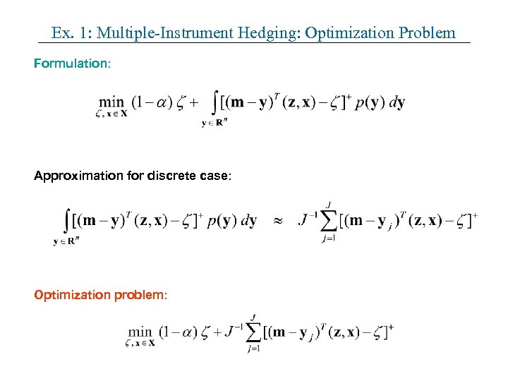Ex. 1: Multiple-Instrument Hedging: Optimization Problem Formulation: Approximation for discrete case: Optimization problem:

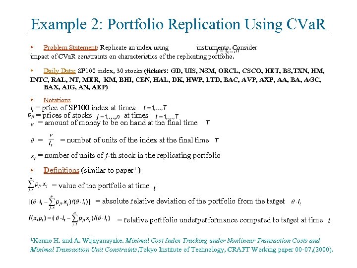Example 2: Portfolio Replication Using CVa. R • Problem Statement: Replicate an index using instruments. Consider impact of CVa. R constraints on characteristics of the replicating portfolio. • Daily Data: SP 100 index, 30 stocks (tickers: GD, UIS, NSM, ORCL, CSCO, HET, BS, TXN, HM, INTC, RAL, NT, MER, KM, BHI, CEN, HAL, DK, HWP, LTD, BAC, AVP, AXP, AA, BA, AGC, BAX, AIG, AN, AEP) • Notations = price of SP 100 index at times = prices of stocks at times = amount of money to be on hand at the final time = = number of units of the index at the final time = number of units of j-th stock in the replicating portfolio • Definitions (similar to paper 1 ) = value of the portfolio at time = absolute relative deviation of the portfolio from the target = relative portfolio underperformance compared to target at time 1 Konno H. and A. Wijayanayake. Minimal Cost Index Tracking under Nonlinear Transaction Costs and Minimal Transaction Unit Constraints, Tokyo Institute of Technology, CRAFT Working paper 00 -07, (2000).

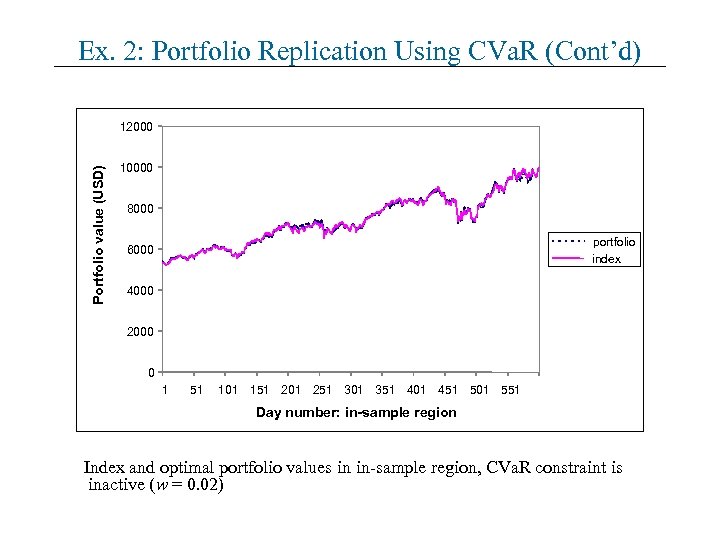Ex. 2: Portfolio Replication Using CVa. R (Cont’d) Portfolio value (USD) 12000 10000 8000 portfolio index 6000 4000 2000 0 1 51 101 151 201 251 301 351 401 451 501 551 Day number: in-sample region Index and optimal portfolio values in in-sample region, CVa. R constraint is inactive (w = 0. 02)

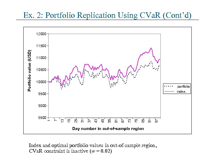Ex. 2: Portfolio Replication Using CVa. R (Cont’d) 12000 Portfolio value (USD) 11500 11000 10500 10000 portfolio index 9500 97 91 85 79 73 67 61 55 49 43 37 31 25 19 13 7 8500 1 9000 Day number in out-of-sample region Index and optimal portfolio values in out-of-sample region, CVa. R constraint is inactive (w = 0. 02)

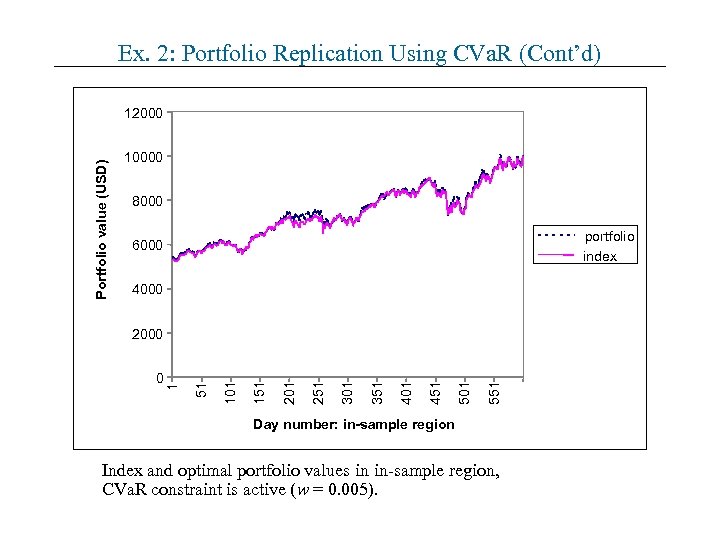Ex. 2: Portfolio Replication Using CVa. R (Cont’d) Portfolio value (USD) 12000 10000 8000 portfolio index 6000 4000 551 501 451 401 351 301 251 201 151 101 51 0 1 2000 Day number: in-sample region Index and optimal portfolio values in in-sample region, CVa. R constraint is active (w = 0. 005).

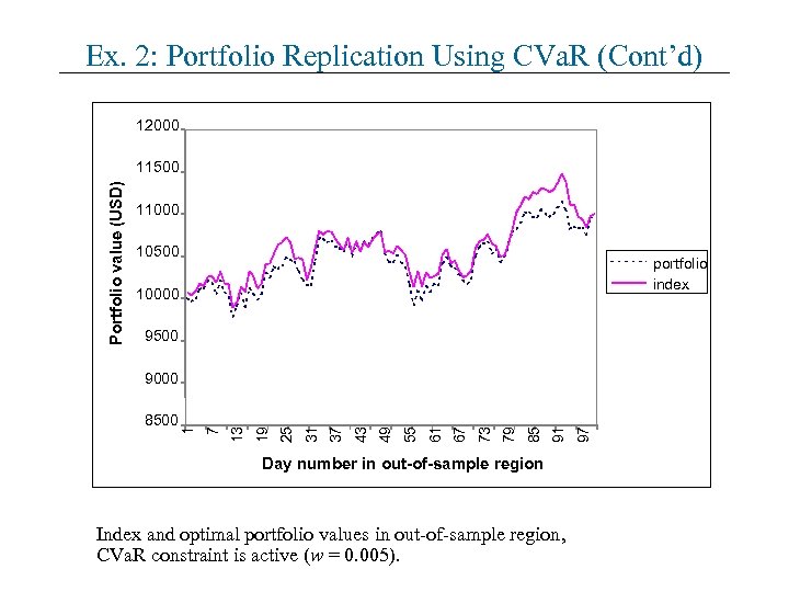Ex. 2: Portfolio Replication Using CVa. R (Cont’d) 12000 Portfolio value (USD) 11500 11000 10500 portfolio index 10000 9500 Day number in out-of-sample region Index and optimal portfolio values in out-of-sample region, CVa. R constraint is active (w = 0. 005). 97 91 85 79 73 67 61 55 49 43 37 31 25 19 13 7 8500 1 9000

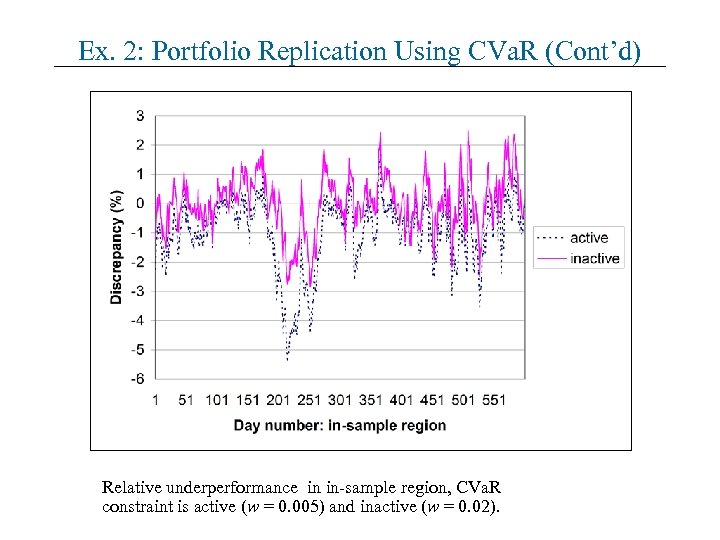Ex. 2: Portfolio Replication Using CVa. R (Cont’d) Relative underperformance in in-sample region, CVa. R constraint is active (w = 0. 005) and inactive (w = 0. 02).

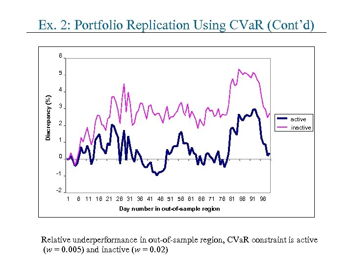Ex. 2: Portfolio Replication Using CVa. R (Cont’d) 6 5 Discrepancy (%) 4 3 active inactive 2 1 0 -1 -2 1 6 11 16 21 26 31 36 41 46 51 56 61 66 71 76 81 86 91 96 Day number in out-of-sample region Relative underperformance in out-of-sample region, CVa. R constraint is active (w = 0. 005) and inactive (w = 0. 02)

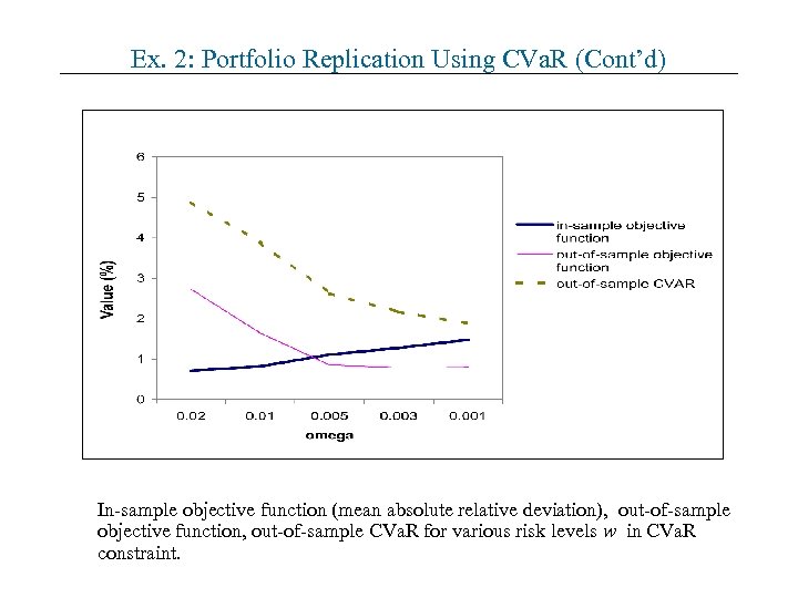Ex. 2: Portfolio Replication Using CVa. R (Cont’d) In-sample objective function (mean absolute relative deviation), out-of-sample objective function, out-of-sample CVa. R for various risk levels w in CVa. R constraint.

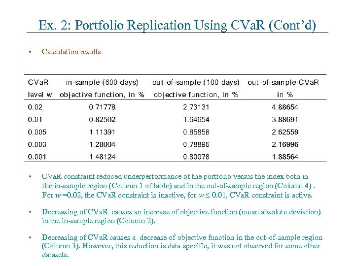Ex. 2: Portfolio Replication Using CVa. R (Cont’d) • Calculation results • CVa. R constraint reduced underperformance of the portfolio versus the index both in the in-sample region (Column 1 of table) and in the out-of-sample region (Column 4). For w =0. 02, the CVa. R constraint is inactive, for w 0. 01, CVa. R constraint is active. • Decreasing of CVa. R causes an increase of objective function (mean absolute deviation) in the in-sample region (Column 2). • Decreasing of CVa. R causes a decrease of objective function in the out-of-sample region (Column 3). However, this reduction is data specific, it was not observed for some other datasets.

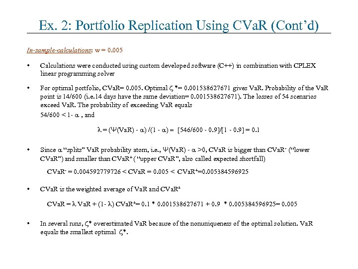Ex. 2: Portfolio Replication Using CVa. R (Cont’d) In-sample-calculations: w = 0. 005 • Calculations were conducted using custom developed software (C++) in combination with CPLEX linear programming solver • For optimal portfolio, CVa. R= 0. 005. Optimal *= 0. 001538627671 gives Va. R. Probability of the Va. R point is 14/600 (i. e. 14 days have the same deviation= 0. 001538627671). The losses of 54 scenarios exceed Va. R. The probability of exceeding Va. R equals 54/600 < 1 - , and = (Ψ(Va. R) - ) /(1 - ) = [546/600 - 0. 9]/[1 - 0. 9] = 0. 1 • Since “splits” Va. R probability atom, i. e. , Ψ(Va. R) - >0, CVa. R is bigger than CVa. R- (“lower CVa. R”) and smaller than CVa. R+ ( “upper CVa. R”, also called expected shortfall) CVa. R- = 0. 004592779726 < CVa. R = 0. 005 < CVa. R+=0. 005384596925 • CVa. R is the weighted average of Va. R and CVa. R+ CVa. R = Va. R + (1 - ) CVa. R+= 0. 1 * 0. 001538627671 + 0. 9 * 0. 005384596925= 0. 005 • In several runs, * overestimated Va. R because of the nonuniqueness of the optimal solution. Va. R equals the smallest optimal *.

Example 3: Asset Liability Management (ALM) Pension Fund Non-Active Members Active members Payments? Future liabilities? Risk Management

Ex. 3: ALM – Data • ORTEC Consultants BV in Holland provided a dataset for a pension fund • 10000 scenarios: liabilities of a fund and returns for 13 assets (indices) • To simplify interpretation of results, mostly, we considered only four assets: 1. cash, 2. Dutch bonds index, 3. European equity index, 4. Dutch real estate index. • However, the approach can easily handle 100, 000 assets.

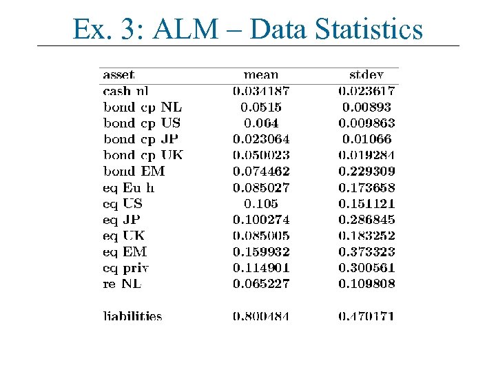Ex. 3: ALM – Data Statistics

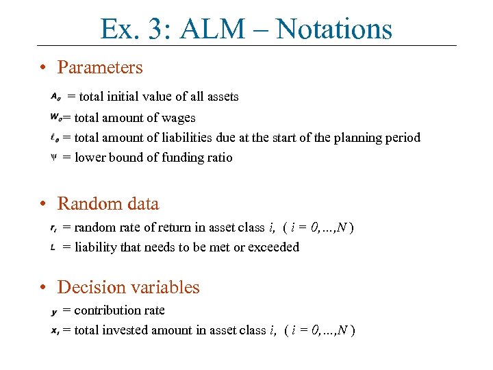Ex. 3: ALM – Notations • Parameters = total initial value of all assets = total amount of wages = total amount of liabilities due at the start of the planning period = lower bound of funding ratio • Random data = random rate of return in asset class i, ( i = 0, …, N ) = liability that needs to be met or exceeded • Decision variables = contribution rate = total invested amount in asset class i, ( i = 0, …, N )

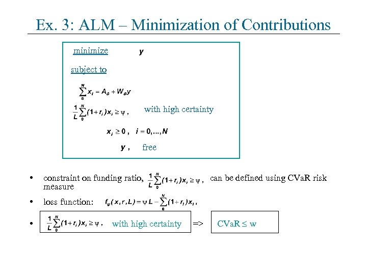Ex. 3: ALM – Minimization of Contributions minimize subject to with high certainty free • constraint on funding ratio, measure • loss function: • with high certainty can be defined using CVa. R risk => CVa. R w

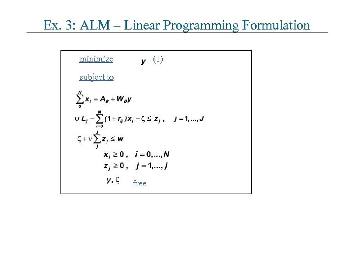Ex. 3: ALM – Linear Programming Formulation minimize (1) subject to free

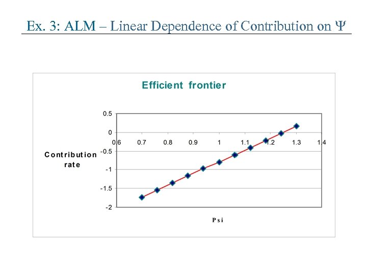
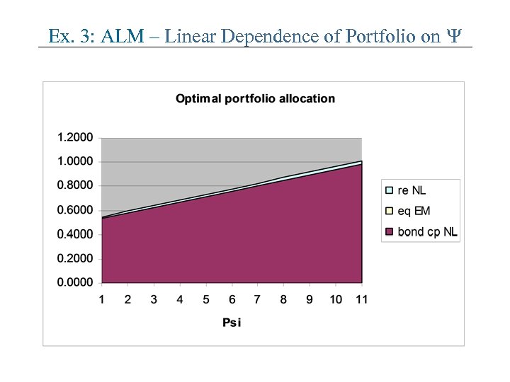
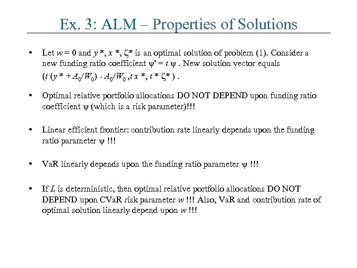Ex. 3: ALM – Properties of Solutions • Let w = 0 and y *, x *, * is an optimal solution of problem (1). Consider a new funding ratio coefficient ' = t . New solution vector equals (t (y * + A 0/W 0) - A 0/W 0 , t x *, t * * ). • Optimal relative portfolio allocations DO NOT DEPEND upon funding ratio coefficient (which is a risk parameter)!!! • Linear efficient frontier: contribution rate linearly depends upon the funding ratio parameter !!! • Va. R linearly depends upon the funding ratio parameter !!! • If L is deterministic, then optimal relative portfolio allocations DO NOT DEPEND upon CVa. R risk parameter w !!! Also, Va. R and contribution rate of optimal solution linearly depend upon w !!!

Ex. 3: ALM – Linear Dependence of Contribution on

Ex. 3: ALM – Linear Dependence of Portfolio on

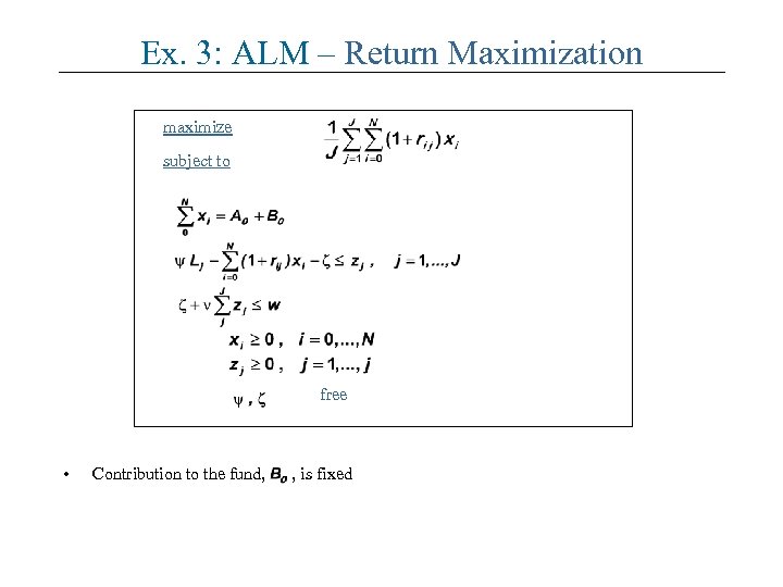Ex. 3: ALM – Return Maximization maximize subject to free • Contribution to the fund, , is fixed

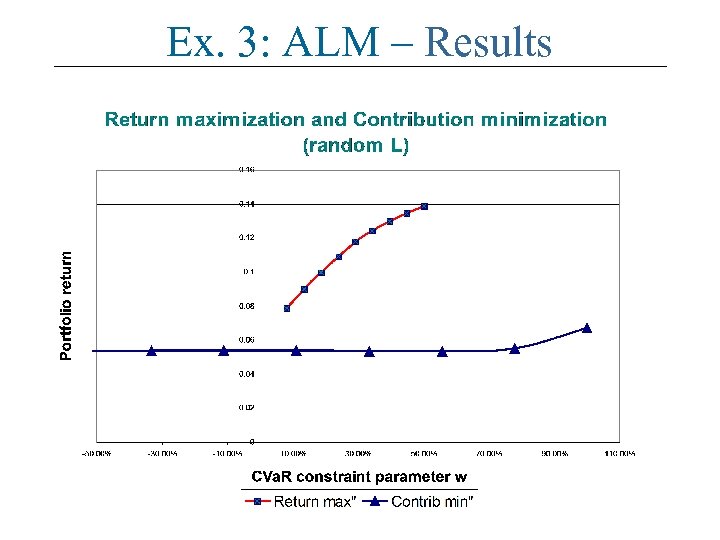Ex. 3: ALM – Results

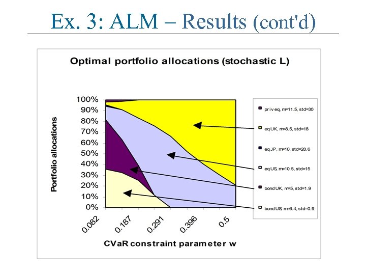Ex. 3: ALM – Results (cont'd)

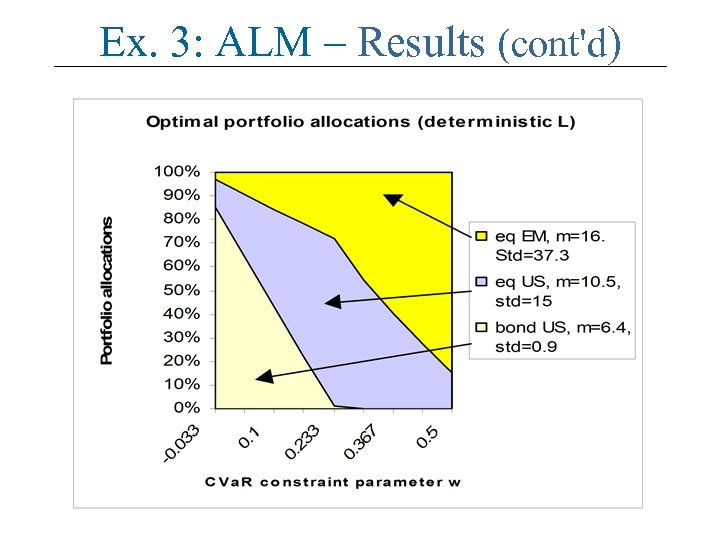Ex. 3: ALM – Results (cont'd)