Stochastic Models for Communication Networks Jean Walrand University

Stochastic Models for Communication Networks Jean Walrand University of California, Berkeley

Contents n Big Picture n n n n 2 Discrete Time DT: LP Formulation Continuous Time Transaction-Level Models n n Little’s Law and Applications Stability of Markov Chains Scheduling Markov Decision Problems n n Store-and-Forward Packets, Transactions, Users Queuing n n (tentative) Models of TCP Stability Random Networks n Connectivity Results: Percolations

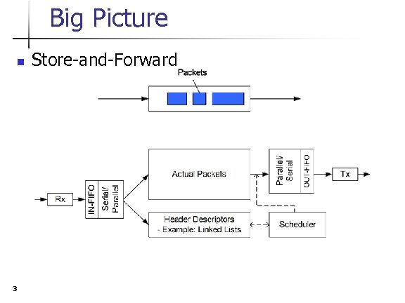Big Picture n 3 Store-and-Forward

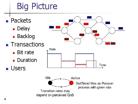Big Picture n Packets n n n Transactions n n n 4 Delay Backlog Bit rate Duration Users

Queuing n n 5 Little’s Law Stability of Markov Chains

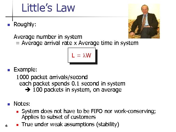Little’s Law n Roughly: Average number in system = Average arrival rate x Average time in system L = l. W n n Example: 1000 packet arrivals/second each packet spends 0. 1 second in system 100 packets in system, on average Notes: n 6 n System does not have to be FIFO nor work-conserving; Applies to subset of customers True under weak assumptions (stability)

Little’s Law… n Extension: Average income per unit time = Average arrival rate x Average cost per customer H = l. G n 7 Example: 1000 customer arrivals/second each customer spends $5. 00 on average system gets $5, 000. 00 per second, on average

Little’s Law… n Illustration 1: Utilization L = l. W H = l. G Packets arrive at rate l (per second) Average transmission time = 1/m (seconds) Transmitter is busy a fraction l/m of the time n 8 Indeed: System = transmitter Number in system = 1 if busy, 0 otherwise W = Average time in system = 1/m L = Average number in system = fraction of time busy Hence, Fraction of time busy = l/m =: link utilization

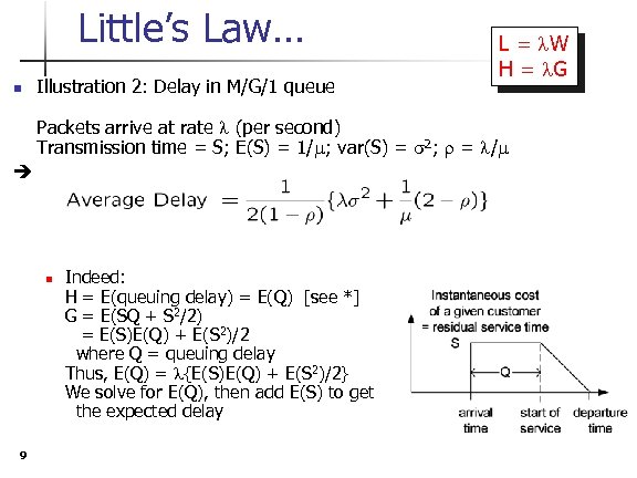Little’s Law… n Illustration 2: Delay in M/G/1 queue L = l. W H = l. G Packets arrive at rate l (per second) Transmission time = S; E(S) = 1/m; var(S) = s 2; r = l/m n 9 Indeed: H = E(queuing delay) = E(Q) [see *] G = E(SQ + S 2/2) = E(S)E(Q) + E(S 2)/2 where Q = queuing delay Thus, E(Q) = l{E(S)E(Q) + E(S 2)/2} We solve for E(Q), then add E(S) to get the expected delay

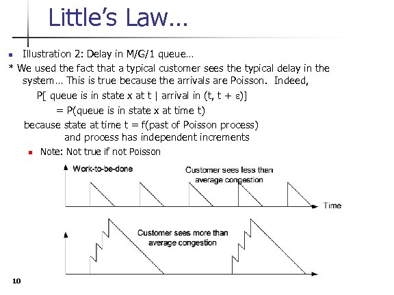Little’s Law… Illustration 2: Delay in M/G/1 queue… * We used the fact that a typical customer sees the typical delay in the system… This is true because the arrivals are Poisson. Indeed, P[ queue is in state x at t | arrival in (t, t + e)] = P(queue is in state x at time t) because state at time t = f(past of Poisson process) and process has independent increments n n 10 Note: Not true if not Poisson

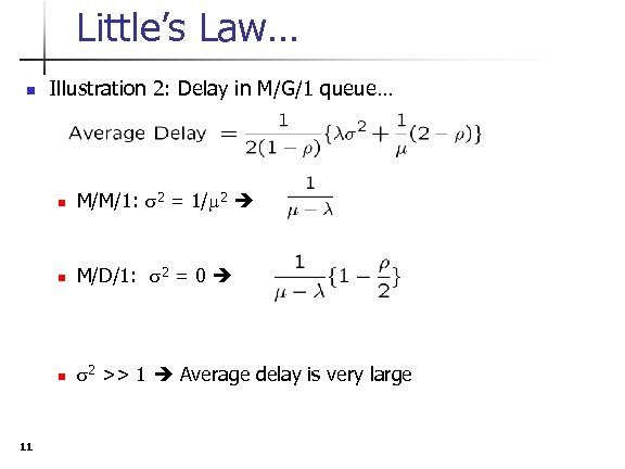Little’s Law… n Illustration 2: Delay in M/G/1 queue… n n M/D/1: s 2 = 0 n 11 M/M/1: s 2 = 1/m 2 s 2 >> 1 Average delay is very large

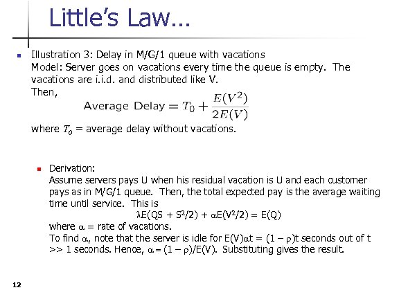Little’s Law… n Illustration 3: Delay in M/G/1 queue with vacations Model: Server goes on vacations every time the queue is empty. The vacations are i. i. d. and distributed like V. Then, where T 0 = average delay without vacations. n 12 Derivation: Assume servers pays U when his residual vacation is U and each customer pays as in M/G/1 queue. Then, the total expected pay is the average waiting time until service. This is l. E(QS + S 2/2) + a. E(V 2/2) = E(Q) where a = rate of vacations. To find a, note that the server is idle for E(V)at = (1 – r)t seconds out of t >> 1 seconds. Hence, a = (1 – r)/E(V). Substituting gives the result.

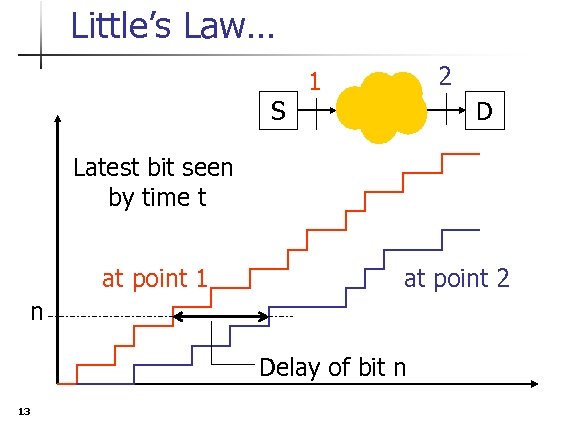Little’s Law… 2 1 S D Latest bit seen by time t at point 1 at point 2 n Delay of bit n 13

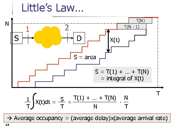Little’s Law… N S 1 T(N) T(N - 1) 2 D X(t) S = area S = T(1) + … + T(N) = integral of X(t) T(1) + … + T(N) N 1 S. X(t)dt = = T T N T T Average occupancy = (average delay)x(average arrival rate) 14

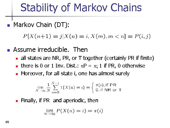Stability of Markov Chains n Markov Chain (DT): n Assume irreducible. Then n all states are NR, PR, or T together (certainly PR if finite) there is 0 or 1 Inv. Dist. : p. P = p; 1 if PR, 0 otherwise Moreover, for all state i, one has almost surely n Finally, if PR and aperiodic, then n n 15

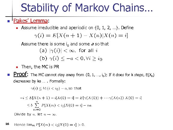Stability of Markov Chains… n Pakes’ Lemma: n Assume irreducible and aperiodic on {0, 1, 2, …}. Define Assume there is some i 0 and some a so that n n Then, the MC is PR Proof: The MC cannot stay away from {0, 1, …, i 0}; If it does for k steps, E(Xn) decreases by ka …. Formally: 16

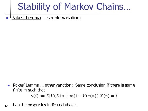Stability of Markov Chains… n n 17 Pakes’ Lemma … simple variation: Pakes’ Lemma … other variation: Same conclusion if there is some finite m such that has the properties indicated above.

Stability of Markov Chains… n Application 1: (Inspired by TCP) First note that X(n) is irreducible and aperiodic. Also, the original form of Pakes’ Lemma applies. 18

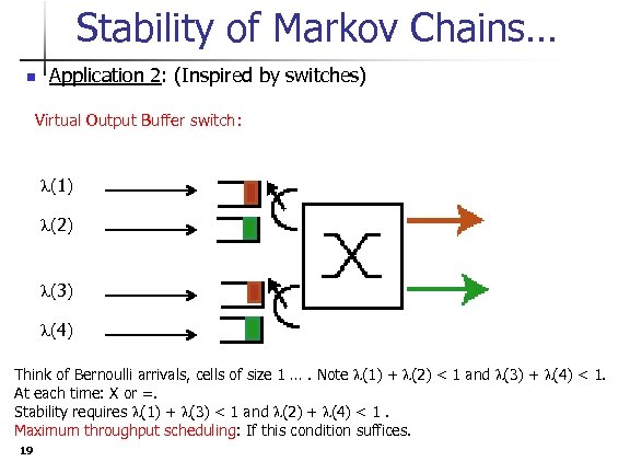Stability of Markov Chains… n Application 2: (Inspired by switches) Virtual Output Buffer switch: l(1) l(2) l(3) l(4) Think of Bernoulli arrivals, cells of size 1 …. Note l(1) + l(2) < 1 and l(3) + l(4) < 1. At each time: X or =. Stability requires l(1) + l(3) < 1 and l(2) + l(4) < 1. Maximum throughput scheduling: If this condition suffices. 19

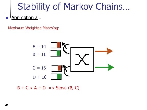Stability of Markov Chains… n Application 2… Maximum Weighted Matching: A = 14 B = 11 C = 15 D = 10 B + C > A + D => Serve (B, C) 20

Stability of Markov Chains… n Application 2 (Tassiulas, Mc. Keown et al) Maximum Weighted Matching maximum throughput. Proof: V(x) = ||x||2 is a Lyapunov function That is, E[V(X(n+1) – V(X(n)) | X(n) = x] is finite and < - e < 0 for x outside a finite set. 21

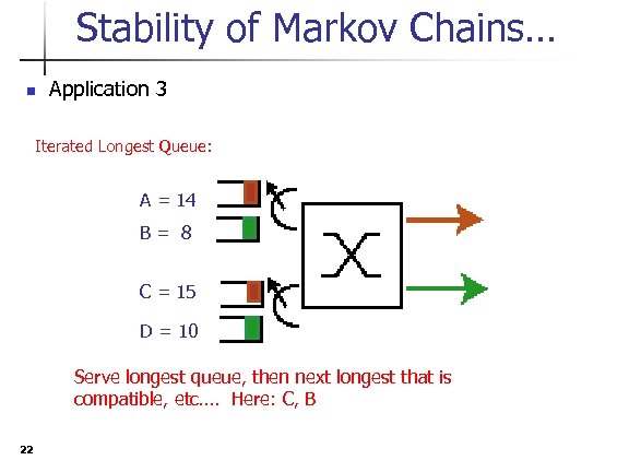Stability of Markov Chains… n Application 3 Iterated Longest Queue: A = 14 B= 8 C = 15 D = 10 Serve longest queue, then next longest that is compatible, etc…. Here: C, B 22

Stability of Markov Chains… n Application 3 (A. Dimakis) Iterated Longest Queue maximum throughput. Proof: V(x) = maxi(xi) is a Lyapunov function. 23

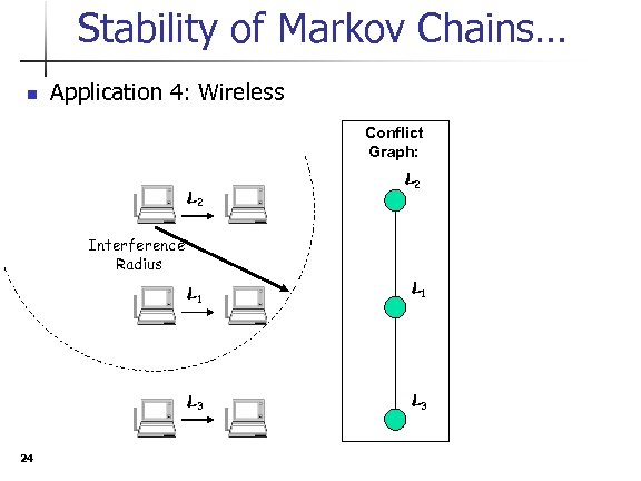Stability of Markov Chains… n Application 4: Wireless Conflict Graph: L 2 Interference Radius L 1 L 3 24 L 1 L 3

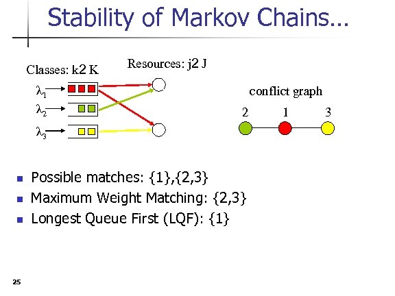Stability of Markov Chains… Classes: k 2 K λ 1 λ 2 Resources: j 2 J conflict graph 2 λ 3 n n n 25 Possible matches: {1}, {2, 3} Maximum Weight Matching: {2, 3} Longest Queue First (LQF): {1} 1 3

Stability of Markov Chains… Iterated Longest Queue maximum throughput. [Dimakis] conflict graph n n 26 As in previous example: n Consider fluid limits; n Use longest queue size as Lyapunov function. Carries over to conflict graph topologies that strictly include trees. n Example: 2 1 3 λ 2 λ 1 λ 3

Stability of Markov Chains… Iterated Longest Queue maximum throughput. 1 2 6 n n 5 3 4 n Nominal stability cnd: li+li+1<1. One fluid limit is unstable for li>3/7* Stochastic system is stable for almost all feasible l’s (A. Dimakis) * Big match is picked 2/3 times in fluid limit when queues are equal, which happens after 3 steps after a small match and 2 steps after a big match. 27

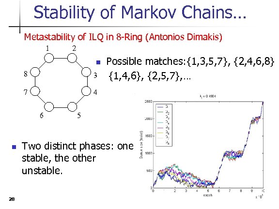Stability of Markov Chains… Metastability of ILQ in 8 -Ring (Antonios Dimakis) 1 2 n 8 3 7 4 6 n 28 Possible matches: {1, 3, 5, 7}, {2, 4, 6, 8} {1, 4, 6}, {2, 5, 7}, … 5 Two distinct phases: one stable, the other unstable.

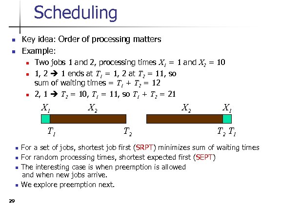Scheduling n n Key idea: Order of processing matters Example: n n n Two jobs 1 and 2, processing times X 1 = 1 and X 2 = 10 1, 2 1 ends at T 1 = 1, 2 at T 2 = 11, so sum of waiting times = T 1 + T 2 = 12 2, 1 T 2 = 10, T 1 = 11, so T 1 + T 2 = 21 X 1 T 1 n n 29 X 2 T 2 X 1 T 2 T 1 For a set of jobs, shortest job first (SRPT) minimizes sum of waiting times For random processing times, shortest expected first (SEPT) The interesting case is when preemption is allowed and when new jobs arrive. We explore preemption next.

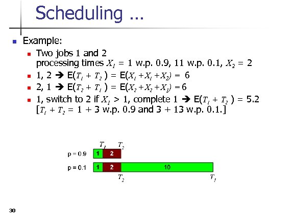Scheduling … n Example: n n 30 Two jobs 1 and 2 processing times X 1 = 1 w. p. 0. 9, 11 w. p. 0. 1, X 2 = 2 1, 2 E(T 1 + T 2 ) = E(X 1 + X 2) = 6 2, 1 E(T 2 + T 1 ) = E(X 2 + X 1) = 6 1, switch to 2 if X 1 > 1, complete 1 E(T 1 + T 2 ) = 5. 2 [T 1 + T 2 = 1 + 3 w. p. 0. 9 and 3 + 13 w. p. 0. 1. ]

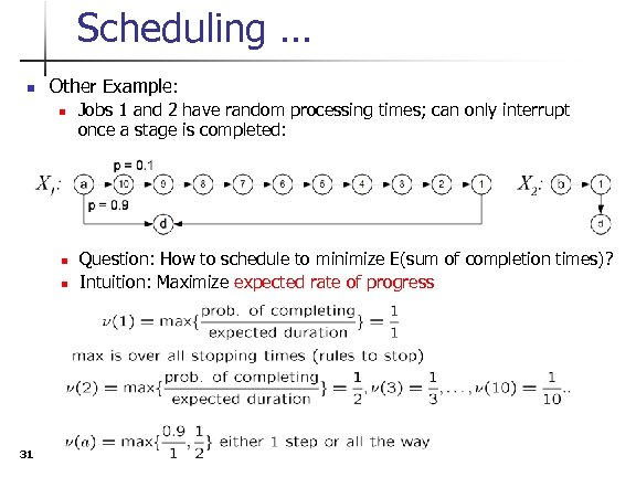Scheduling … n Other Example: n n n 31 Jobs 1 and 2 have random processing times; can only interrupt once a stage is completed: Question: How to schedule to minimize E(sum of completion times)? Intuition: Maximize expected rate of progress

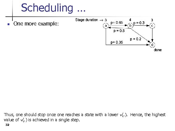Scheduling … n One more example: Thus, one should stop once one reaches a state with a lower n(. ). Hence, the highest value of n(. ) is achieved in a single step. 32

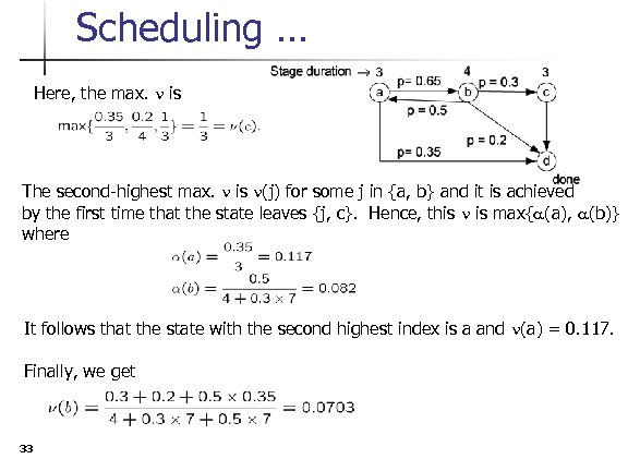Scheduling … Here, the max. n is The second-highest max. n is n(j) for some j in {a, b} and it is achieved by the first time that the state leaves {j, c}. Hence, this n is max{a(a), a(b)} where It follows that the state with the second highest index is a and n(a) = 0. 117. Finally, we get 33

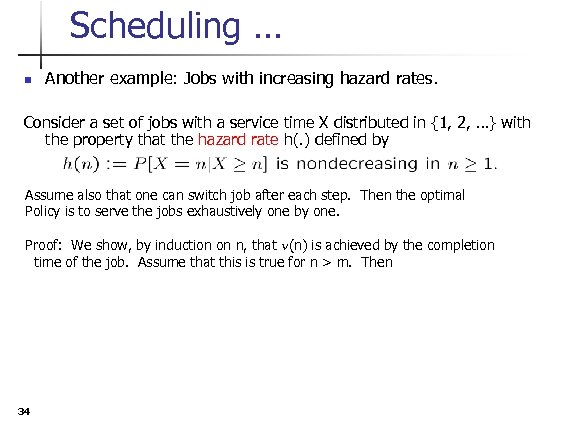Scheduling … n Another example: Jobs with increasing hazard rates. Consider a set of jobs with a service time X distributed in {1, 2, …} with the property that the hazard rate h(. ) defined by Assume also that one can switch job after each step. Then the optimal Policy is to serve the jobs exhaustively one by one. Proof: We show, by induction on n, that n(n) is achieved by the completion time of the job. Assume that this is true for n > m. Then 34

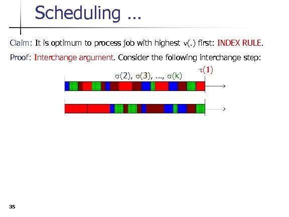Scheduling … Claim: It is optimum to process job with highest n(. ) first: INDEX RULE. Proof: Interchange argument. Consider the following interchange step: t(1) s(2), s(3), …, s(k) 35

Markov Decision Problems n n n 36 Objective: How to make decisions in face of uncertainty Example: Guessing next card Example: Serving queues Discrete-Time Formulation Continuous-Time Formulation Linear Programming Formulation

Markov Decision Problems n Decision in the face of uncertainty n n n 37 Should you carry an umbrella? Should get vaccinated against the flu? Take another card at blackjack? Buy a lottery ticket Fill up at the next gas station? Guess that the transmitter sent a 1? Take the prelims next time? Stay on for a Ph. D? Marry my boyfriend? Choose another advisor? Drop out of this silly course? ….

Markov Decision Problems n Example (from S. Ross “Introduction to Stochastic Dynamic Programming”) n n n A perfectly shuffled deck of 52 cards Guess once if next card is an ace: + $10. 00 if correct; $ 0. 00 if not. Can decide when to bet on the next card. You see the cards as they are being turned over. Optimal policy: Any guess is correct as long as there is still an ace in the deck. Proof: n n 38 Let V(n, m) be the best chance of guessing correctly if there are still n cards with m aces in the deck (0 <= m <= n). Then V satisfies the following Dynamic Programming Equations:

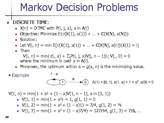Markov Decision Problems n DISCRETE TIME: n n n X(n) = DTMC with P(i, j, a), a in A(i) Objective: Minimize E{c(X(1), a(1)) + … + C(X(N), a(N))} Solution: Let V(i, n) = min E[c(X(1), a(1)) + … + C(X(N), a(n))|X(1) = i] Then V(i, n) = min{c(i, a) + Sj. P(i, j, a)V(j, n – 1)}; V(. , 0) = 0 where the minimum is over a in A(i). Moreover, the optimum action a = g(x, n) is the minimizing value. • Example V(1, n) = min{1 + a 2 + (1 – a)V(1, n – 1), a in [0, 1]} n V(1, 1) = min{1 + a 2} = 1, g(1, 1) = 0 n V(1, 2) = min{1 + a 2 + (1 – a)1} = 7/4, g(1, 2) = ½ n V(1, 3) = min{1 + a 2 + (1 – a)7/4} = 127/64, g(1, 3) = 7/8, … 39

Markov Decision Problems n DISCRETE TIME: Average cost n n X(n) = DTMC with P(i, j, a), a in A(i) Objective: Minimize E{c(X, a(X)) } where X is invariant under P(i, j, a(i)) Solution: Roughly, V(i, n) = n. V + h(i), so that n. V + h(i) = min{c(i, a) + (n – 1)V + Sj. P(i, j, a)h(j)} Hence, V + h(i) = min{c(i, a) + 40 Sj. P(i, j, a)h(j)}

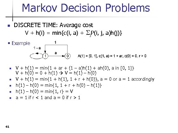Markov Decision Problems n DISCRETE TIME: Average cost V + h(i) = min{c(i, a) + Sj. P(i, j, a)h(j)} • Example n n n 41 V + h(1) = min{1 + ar + (1 – a)h(1) + ah(0), a in [0, 1]} V + h(0) = 0 + h(1) V = h(1) – h(0) V + h(1) = min{1 + h(1), 1 + r + h(0)}, a = 0 or a = 1 accordingly h(1) – h(0) = min{1, 1 + r + h(0) – h(1)} h(1) – h(0) = min{1, r} = V a = 1 if r < 1 and a = 0 if r > 1

Markov Decision Problems n 42 DISCRETE TIME: Average Cost - Linear Programming