Stochastic Dynamic Programming Review DP with

Stochastic Dynamic Programming – Review – DP with probabilities 1 MIT and James Orlin © 2003

Overview Objective: illustrate the use of DP with probabilities l Seems more complex because it is a more complex decision at each stage l But the optimal decision at each stage still depends on the previous stages. l 2 MIT and James Orlin © 2003

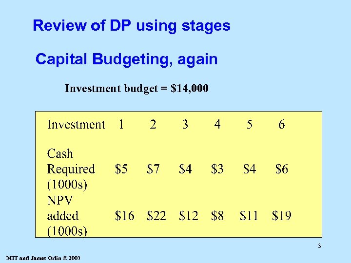Review of DP using stages Capital Budgeting, again Investment budget = $14, 000 3 MIT and James Orlin © 2003

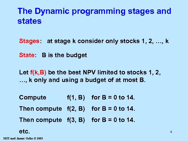The Dynamic programming stages and states Stages: at stage k consider only stocks 1, 2, …, k State: B is the budget Let f(k, B) be the best NPV limited to stocks 1, 2, …, k only and using a budget of at most B. Compute f(1, B) for B = 0 to 14. Then compute f(2, B) for B = 0 to 14. Then compute f(3, B) for B = 0 to 14. etc. MIT and James Orlin © 2003 4

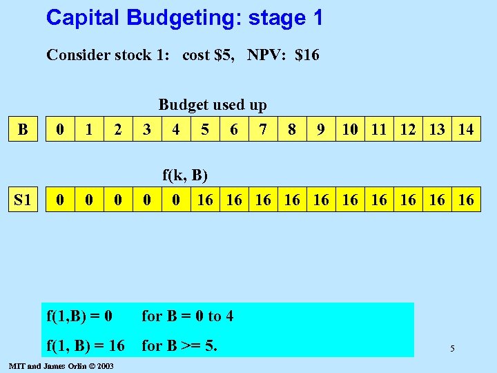Capital Budgeting: stage 1 Consider stock 1: cost $5, NPV: $16 B S 1 0 0 1 0 2 Budget used up 3 4 5 6 7 0 f(k, B) 0 0 16 16 16 f(1, B) = 0 for B >= 5. 9 10 11 12 13 14 for B = 0 to 4 f(1, B) = 16 8 MIT and James Orlin © 2003 5

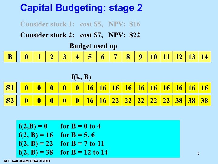Capital Budgeting: stage 2 Consider stock 1: cost $5, NPV: $16 Consider stock 2: cost $7, NPV: $22 B 0 1 2 Budget used up 3 4 5 6 7 8 9 10 11 12 13 14 S 1 0 0 0 f(k, B) 0 0 16 16 16 S 2 0 0 f(2, B) = 16 f(2, B) = 22 f(2, B) = 38 MIT and James Orlin © 2003 0 16 16 22 22 22 38 38 38 for B = 0 to 4 for B = 5, 6 for B = 7 to 11 for B = 12 to 14 6

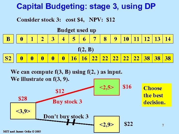Capital Budgeting: stage 3, using DP Consider stock 3: cost $4, NPV: $12 Budget used up B 0 S 2 0 1 0 2 0 3 0 4 5 6 7 8 9 10 11 12 13 14 0 f(2, B) 16 16 22 22 22 38 38 38 We can compute f(3, B) using f(2, ) as input. We illustrate on f(3, 9). <2, 5> $16 $12 $28 Buy stock 3 <3, 9> Don’t buy stock 3 <2, 9> MIT and James Orlin © 2003 Choose the best decision. $22 7

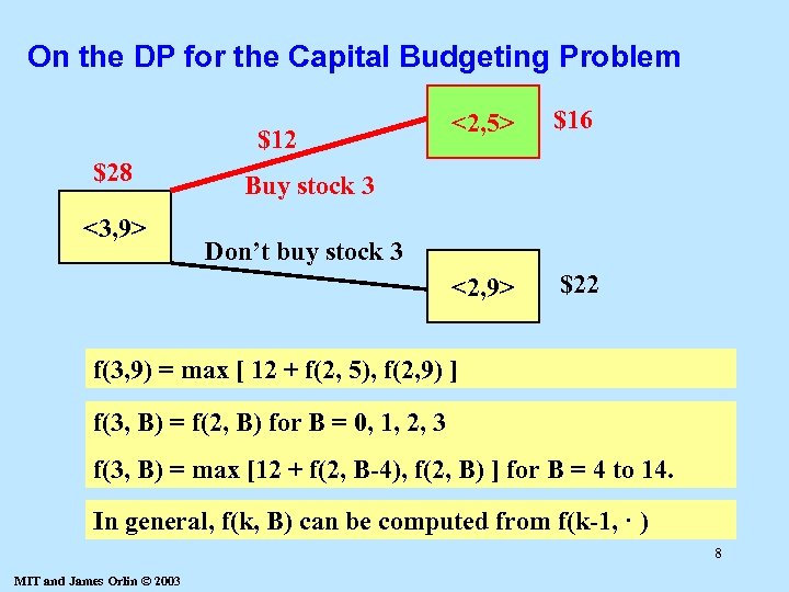On the DP for the Capital Budgeting Problem $28 <3, 9> $16 <2, 9> $12 <2, 5> $22 Buy stock 3 Don’t buy stock 3 f(3, 9) = max [ 12 + f(2, 5), f(2, 9) ] f(3, B) = f(2, B) for B = 0, 1, 2, 3 f(3, B) = max [12 + f(2, B-4), f(2, B) ] for B = 4 to 14. In general, f(k, B) can be computed from f(k-1, · ) 8 MIT and James Orlin © 2003

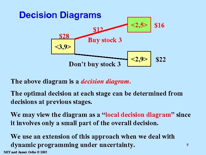Decision Diagrams $28 <3, 9> $12 <2, 5> $16 Buy stock 3 Don’t buy stock 3 <2, 9> $22 The above diagram is a decision diagram. The optimal decision at each stage can be determined from decisions at previous stages. We may view the diagram as a “local decision diagram” since it involves only a small part of the overall decision. We use an extension of this approach when we deal with dynamic programming under uncertainty. MIT and James Orlin © 2003 9

Dynamic Programming under uncertainty l Next: we will permit uncertainties in our DPs. l This is usually where DP gets much more powerful as a tool, but also more complex l We illustrate with an example in warfare, or gaming if you prefer. 10 MIT and James Orlin © 2003

Destroying an enemy target: a bomber example l You are a pilot in enemy territory. Your mission is to destroy an important target. You must get through. You have four minutes to reach your target, and have just been spotted by radar. l Enemies have can launch up to one bomber per minute to prevent you from reaching the target. The probability of them launching a bomber in any minute is qi for i = 1 to 4. 11 MIT and James Orlin © 2003

A bomber example, continued l To protect yourself, you have M missiles. Each has a probability of pj of destroying the bomber. l Whenever you see a bomber, you must decide how many missiles to launch. If you do not destroy the bomber, then you will be destroyed. l Determine a strategy for how many missiles to launch at each time, assuming you see a bomber attacking you. – Let f(k, m) be the number of missiles to launch assuming that you have k minutes left and have m missiles on hand. – A strategy is to determine f(k, m) for k = 1 to 4 and m = 1 to M. 12 MIT and James Orlin © 2003

Simulating the bomber example l Each person has a die and a page describing the probabilities. l Simulate 1 or more instances of the game. – We will discuss the results – Then we will show to determine an optimal strategy using DP 13 MIT and James Orlin © 2003

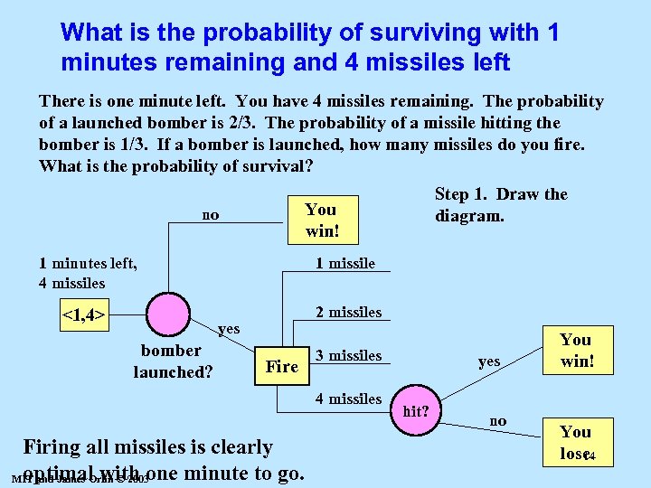What is the probability of surviving with 1 minutes remaining and 4 missiles left There is one minute left. You have 4 missiles remaining. The probability of a launched bomber is 2/3. The probability of a missile hitting the bomber is 1/3. If a bomber is launched, how many missiles do you fire. What is the probability of survival? Step 1. Draw the diagram. You win! no 1 minutes left, 4 missiles 1 missile <1, 4> 2 missiles yes bomber launched? Fire 3 missiles 4 missiles Firing all missiles is clearly optimal with one minute to go. MIT and James Orlin © 2003 yes hit? no You win! You lose. 14

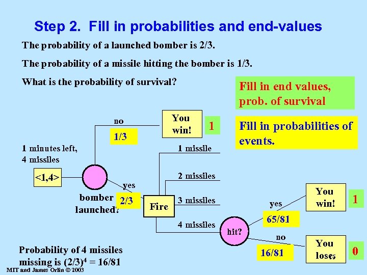Step 2. Fill in probabilities and end-values The probability of a launched bomber is 2/3. The probability of a missile hitting the bomber is 1/3. What is the probability of survival? Fill in end values, prob. of survival You win! no 1/3 1 1 minutes left, 4 missiles 1 missile <1, 4> Fill in probabilities of events. 2 missiles yes bomber 2/3 launched? Fire 3 missiles 4 missiles Probability of 4 missiles missing is (2/3)4 = 16/81 MIT and James Orlin © 2003 yes You win! 1 You lose. 15 0 65/81 hit? no 16/81

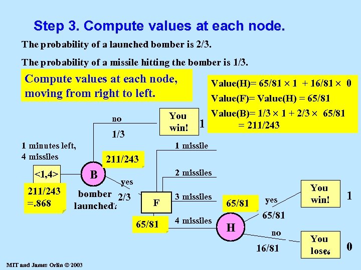Step 3. Compute values at each node. The probability of a launched bomber is 2/3. The probability of a missile hitting the bomber is 1/3. Compute values at each node, moving from right to left. You win! no 1/3 1 minutes left, 4 missiles 211/243 =. 868 1 missile 211/243 B <1, 4> 1 Value(H)= 65/81 1 + 16/81 0 Value(F)= Value(H) = 65/81 Value(B)= 1/3 1 + 2/3 65/81 = 211/243 2 missiles yes bomber 2/3 launched? F 65/81 3 missiles 4 missiles 65/81 yes 1 You lose. 16 0 65/81 H no 16/81 MIT and James Orlin © 2003 You win!

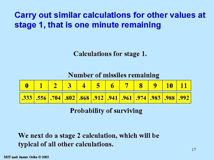Carry out similar calculations for other values at stage 1, that is one minute remaining Calculations for stage 1. 0 1 2 Number of missiles remaining 3 4 5 6 7 8 9 10 11 . 333. 556. 704. 802. 868. 912. 941. 961. 974. 983. 988. 992 Probability of surviving We next do a stage 2 calculation, which will be typical of all other calculations. MIT and James Orlin © 2003 17

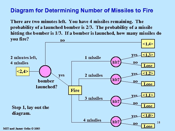Diagram for Determining Number of Missiles to Fire There are two minutes left. You have 4 missiles remaining. The probability of a launched bomber is 2/3. The probability of a missile hitting the bomber is 1/3. If a bomber is launched, how many missiles do you fire? no <1, 4> 2 minutes left, 4 missiles <2, 4> 1 missile yes bomber launched? 2 missiles yes hit? Fire 3 missiles MIT and James Orlin © 2003 no yes hit? Step 1, lay out the diagram. 4 missiles no no yes hit? no <1, 3> Lose <1, 2> Lose <1, 1> Lose <1, 0> Lose 18

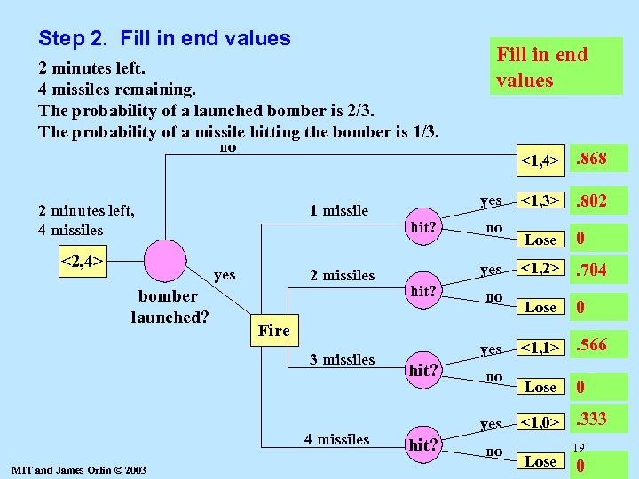Step 2. Fill in end values 2 minutes left. 4 missiles remaining. The probability of a launched bomber is 2/3. The probability of a missile hitting the bomber is 1/3. Fill in end values no <1, 4> 2 minutes left, 4 missiles <2, 4> 1 missile yes bomber launched? 2 missiles hit? 4 missiles no yes hit? Fire 3 missiles MIT and James Orlin © 2003 yes no yes hit? no . 868 <1, 3> . 802 Lose 0 <1, 2> . 704 Lose 0 <1, 1> . 566 Lose 0 <1, 0> . 333 Lose 19 0

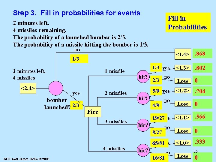Step 3. Fill in probabilities for events Fill in Probabilities 2 minutes left. 4 missiles remaining. The probability of a launched bomber is 2/3. The probability of a missile hitting the bomber is 1/3. no <1, 4> 1/3 2 minutes left, 4 missiles <2, 4> 1 missile yes bomber launched? 2/3 2 missiles 1/3 yes hit? 2/3 5/9 yes hit? 4/9 Fire 3 missiles MIT and James Orlin © 2003 no 19/27 yes hit? 8/27 4 missiles no no 65/81 yes hit? no 16/81 . 868 <1, 3> . 802 Lose 0 <1, 2> . 704 Lose 0 <1, 1> . 566 Lose 0 <1, 0> . 333 Lose 20 0

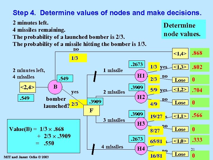Step 4. Determine values of nodes and make decisions. 2 minutes left. 4 missiles remaining. The probability of a launched bomber is 2/3. The probability of a missile hitting the bomber is 1/3. Determine node values. no <1, 4> 1/3. 2673 2 minutes left, 4 missiles . 549 B <2, 4>. 549 1 missile yes bomber launched? 2/3 Value(F) = Value(B) = 1/3 . 704 Value(H 4) Value(H 3) 65/81. 802 Value(H 2) 19/27 . 333 Value(H 1) =1/3 . 868. 566 5/9 max[Value(H 1), Value(H 2), + 16/81 00 ++2/3 . 3909 2/3 0 8/27 4/9 Value(H 3), Value(H 4)] =. 2673 =. 550 =. 3909 MIT and James Orlin © 2003 2 missiles. 3909 H 1. 3909 1/3 yes 2/3 5/9 yes H 2 4/9 F . 3909 3 missiles 8/27 4 missiles H 4 no 19/27 yes H 3. 2673 no no 65/81 yes no 16/81 . 868 <1, 3> . 802 Lose 0 <1, 2> . 704 Lose 0 <1, 1> . 566 Lose 0 <1, 0> . 333 Lose 21 0

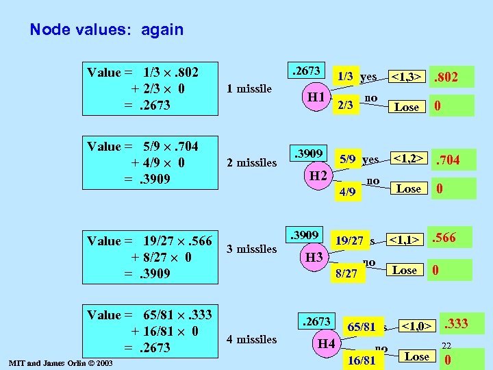Node values: again Value = 1/3 . 802 + 2/3 0 =. 2673 1 missile Value = 5/9 . 704 + 4/9 0 =. 3909 2 missiles Value = 19/27 . 566 + 8/27 0 =. 3909 Value = 65/81 . 333 + 16/81 0 =. 2673 MIT and James Orlin © 2003 . 2673 H 1 . 3909 1/3 yes 2/3 5/9 yes H 2 4/9. 3909 3 missiles 8/27 4 missiles H 4 no 19/27 yes H 3 . 2673 no no 65/81 yes no 16/81 <1, 3> . 802 Lose 0 <1, 2> . 704 Lose 0 <1, 1> . 566 Lose 0 <1, 0> Lose . 333 22 0

Some comments on DP l Seems complex, but the computations are all very similar. – easy to program (not so easy in Excel) – very efficient Useful in finance – investments over time – the outcome of an investment is uncertain l Useful in inventory control – demands are uncertain – supplies must be ordered in advance l 23 MIT and James Orlin © 2003

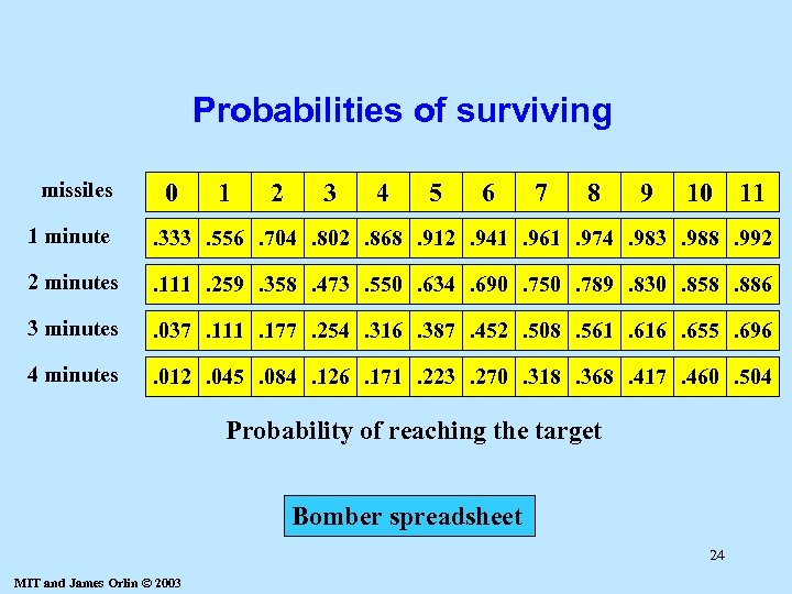Probabilities of surviving missiles 0 1 2 3 4 5 6 7 8 9 10 11 1 minute . 333. 556. 704. 802. 868. 912. 941. 961. 974. 983. 988. 992 2 minutes . 111. 259. 358. 473. 550. 634. 690. 750. 789. 830. 858. 886 3 minutes . 037. 111. 177. 254. 316. 387. 452. 508. 561. 616. 655. 696 4 minutes . 012. 045. 084. 126. 171. 223. 270. 318. 368. 417. 460. 504 Probability of reaching the target Bomber spreadsheet 24 MIT and James Orlin © 2003

Summary for dynamic programming l l l Useful in decision making over time Uses stages, states, optimal value functions Uses recursion Can incorporate probabilities Useful in inventory management, finance, shortest path, and much more 25 MIT and James Orlin © 2003