62cd69df443efe7c97c43312d616dfcb.ppt
- Количество слайдов: 66
 Statistical Methods Allen’s Chapter 7 J&M’s Chapters 8 and 12 1
 Statistical Methods • Large data sets (Corpora) of natural languages allow using statistical methods that were not possible before • Brown Corpus includes about 1000000 words with POS • Penn Treebank contains full syntactic annotations 2
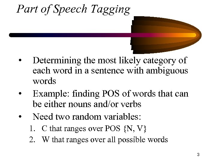 Part of Speech Tagging • • • Determining the most likely category of each word in a sentence with ambiguous words Example: finding POS of words that can be either nouns and/or verbs Need two random variables: 1. C that ranges over POS {N, V} 2. W that ranges over all possible words 3
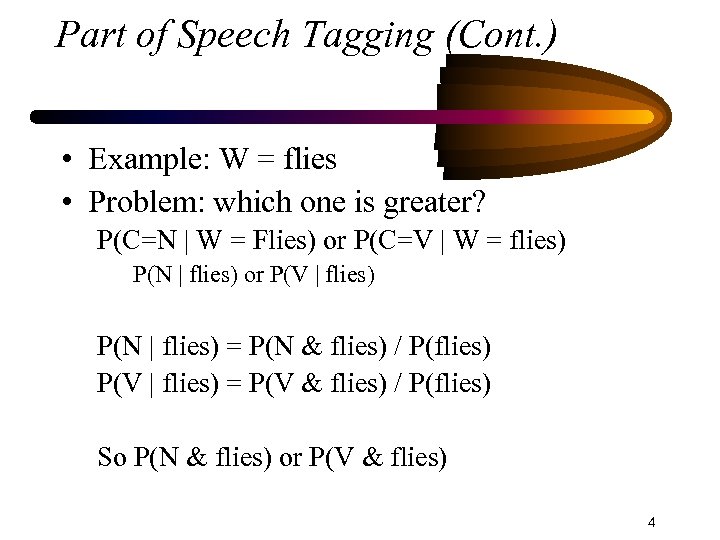 Part of Speech Tagging (Cont. ) • Example: W = flies • Problem: which one is greater? P(C=N | W = Flies) or P(C=V | W = flies) P(N | flies) or P(V | flies) P(N | flies) = P(N & flies) / P(flies) P(V | flies) = P(V & flies) / P(flies) So P(N & flies) or P(V & flies) 4
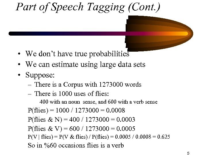 Part of Speech Tagging (Cont. ) • We don’t have true probabilities • We can estimate using large data sets • Suppose: – There is a Corpus with 1273000 words – There is 1000 uses of flies: 400 with an noun sense, and 600 with a verb sense P(flies) = 1000 / 1273000 = 0. 0008 P(flies & N) = 400 / 1273000 = 0. 0003 P(flies & V) = 600 / 1273000 = 0. 0005 P(V | flies) = P(V & flies) / P(flies) = 0. 0005 / 0. 0008 = 0. 625 So in %60 occasions flies is a verb 5
 Estimating Probabilities • We want to use probability to predict the future events • Using the information P(V | flies) = 0. 625 to predict that the next “flies” is more likely to be a verb • This is called Maximum Likelihood estimation (MLE) • Generally the larger the data set we use, the more accuracy we get 6
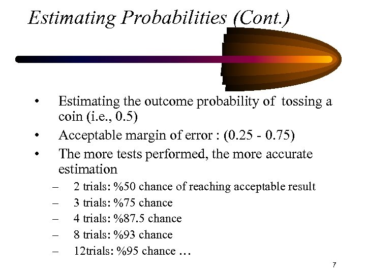 Estimating Probabilities (Cont. ) • • • Estimating the outcome probability of tossing a coin (i. e. , 0. 5) Acceptable margin of error : (0. 25 - 0. 75) The more tests performed, the more accurate estimation – – – 2 trials: %50 chance of reaching acceptable result 3 trials: %75 chance 4 trials: %87. 5 chance 8 trials: %93 chance 12 trials: %95 chance … 7
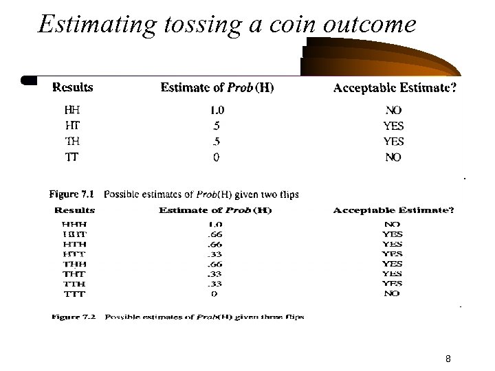 Estimating tossing a coin outcome 8
 Estimating Probabilities (Cont. ) • So the larger data set the better, but • The problem of sparse data • Brown Corpus contains about a million words – but there is only 49000 different words, – so one expect each word occurs about 20 times, – But over 40000 words occur less than 5 times. 9
 Estimating Probabilities (Cont. ) • For a random variable X with a set of values Vi, computed from counting number times X = xi • P(X = xi) Vi / i Vi • Maximum Likelihood Estimation (MLE) uses Vi = |xi| • Expected likelihood Estimation (ELE) Uses Vi = |xi| + 0. 5 10
 MLE vs ELE • Suppose a word w doesn’t occur in the Corpus • We want to estimate w occurring in one of 40 classes L 1 … L 40 • We have a random variable X, • X = xi only if w appears in word category Li • By MLE, P(Li | w) is undefined because the divisor is zero • ELE , P(Li | w) 0. 5 / 20 = 0. 025 • Suppose w occurs 5 times (4 times as an noun and once as a verb) • By MLE, P(N |w) = 4/5 = 0. 8, • By ELE, P(N | w) =4. 5/25 = 0. 18 11
 Evaluation • Data set is divided into: – Training set (%80 -%90 of the data) – Test set (%10 -%20) • Cross-Validation: – Repeatedly removing different parts of corpus as the test set, – Training on the reminder of the corpus, – Then evaluating the new test set. 12
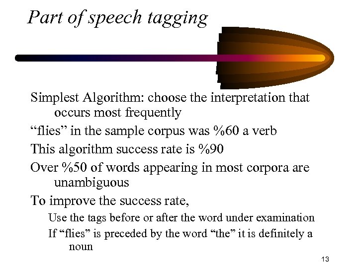 Part of speech tagging Simplest Algorithm: choose the interpretation that occurs most frequently “flies” in the sample corpus was %60 a verb This algorithm success rate is %90 Over %50 of words appearing in most corpora are unambiguous To improve the success rate, Use the tags before or after the word under examination If “flies” is preceded by the word “the” it is definitely a noun 13
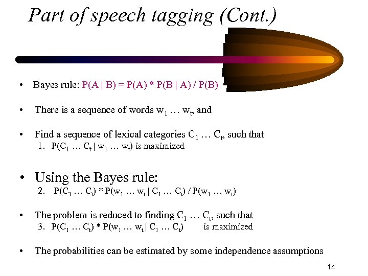 Part of speech tagging (Cont. ) • Bayes rule: P(A | B) = P(A) * P(B | A) / P(B) • There is a sequence of words w 1 … wt, and • Find a sequence of lexical categories C 1 … Ct, such that 1. P(C 1 … Ct | w 1 … wt) is maximized • Using the Bayes rule: 2. P(C 1 … Ct) * P(w 1 … wt | C 1 … Ct) / P(w 1 … wt) • The problem is reduced to finding C 1 … Ct, such that 3. P(C 1 … Ct) * P(w 1 … wt | C 1 … Ct) • is maximized The probabilities can be estimated by some independence assumptions 14
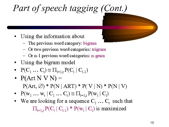 Part of speech tagging (Cont. ) • Using the information about – The previous word category: bigram – Or two previous word categories: trigram – Or n-1 previous word categories: n-gram • Using the bigram model • P(C 1 … Ct) i=1, t P(Ci | Ci-1) • P(Art N V N) = P(Art, ) * P(N | ART) * P( V | N) * P(N | V) • P(w 1 … wt | C 1 … Ct) i=1, t P(wi | Ci) • We are looking for a sequence C 1 … Ct such that i=1, t P(Ci | Ci-1) * P(wi | Ci) is maximized 15
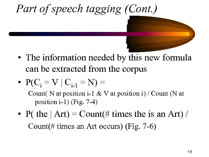 Part of speech tagging (Cont. ) • The information needed by this new formula can be extracted from the corpus • P(Ci = V | Ci-1 = N) = Count( N at position i-1 & V at position i) / Count (N at position i-1) (Fig. 7 -4) • P( the | Art) = Count(# times the is an Art) / Count(# times an Art occurs) (Fig. 7 -6) 16
 Using an Artificial corpus • An artificial corpus generated with 300 sentences of categories Art, N, V, P • 1998 words, 833 nouns, 300 verbs, 558 article, and 307 propositions, • To deal with the problem of the sparse data, a minimum probability of 0. 0001 is assumed 17
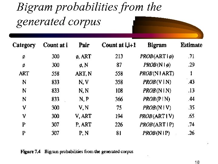 Bigram probabilities from the generated corpus 18
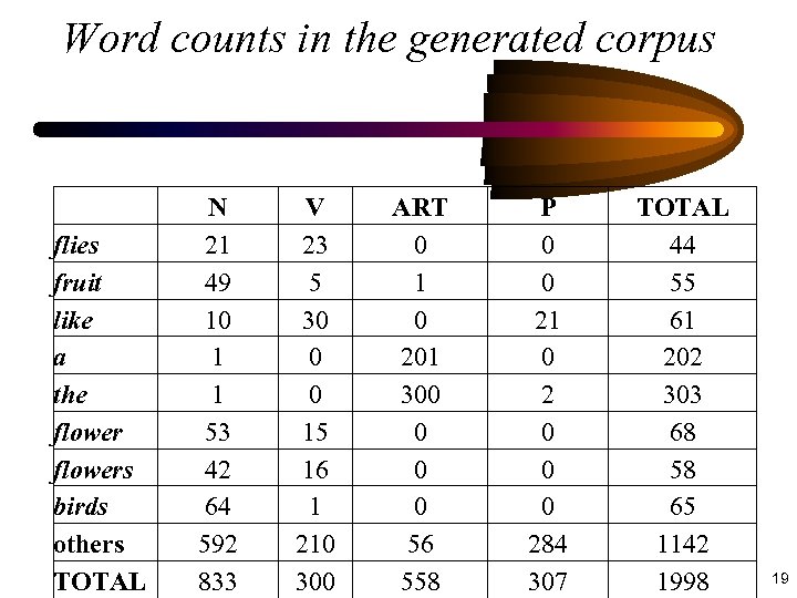 Word counts in the generated corpus flies fruit like a the flowers birds others TOTAL N 21 49 10 1 1 53 42 64 592 833 V 23 5 30 0 0 15 16 1 210 300 ART 0 1 0 201 300 0 56 558 P 0 0 21 0 2 0 0 0 284 307 TOTAL 44 55 61 202 303 68 58 65 1142 1998 19
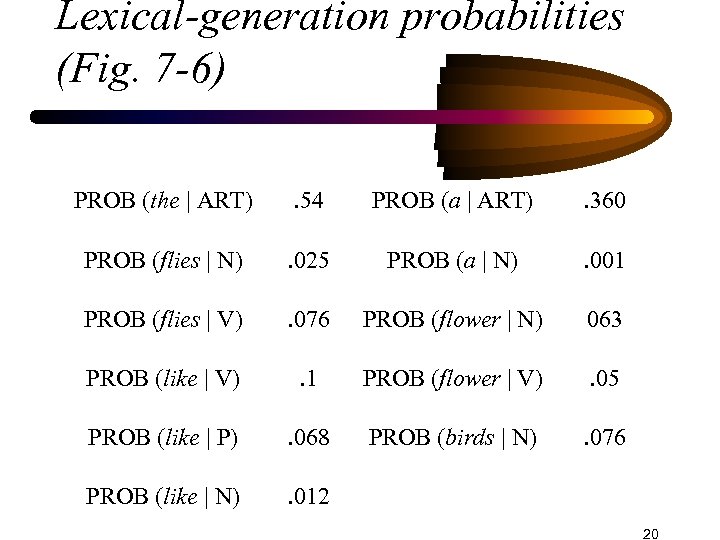 Lexical-generation probabilities (Fig. 7 -6) PROB (the | ART) . 54 PROB (a | ART) . 360 PROB (flies | N) . 025 PROB (a | N) . 001 PROB (flies | V) . 076 PROB (flower | N) 063 PROB (like | V) . 1 PROB (flower | V) . 05 PROB (like | P) . 068 PROB (birds | N) . 076 PROB (like | N) . 012 20
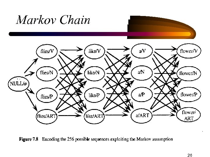
 Part of speech tagging (Cont. ) • How to find the sequence C 1 … Ct that maximizes i=1, t P(Ci | Ci-1) * P(wi | Ci) • Brute Force search: Finding all possible sequences With N categories and T words, there are NT sequences • Using bigram probabilities, the probability wi to be in category Ci depends only on Ci-1 • The process can be modeled by a special form of probabilistic finite state machine (Fig. 7 -7) 21
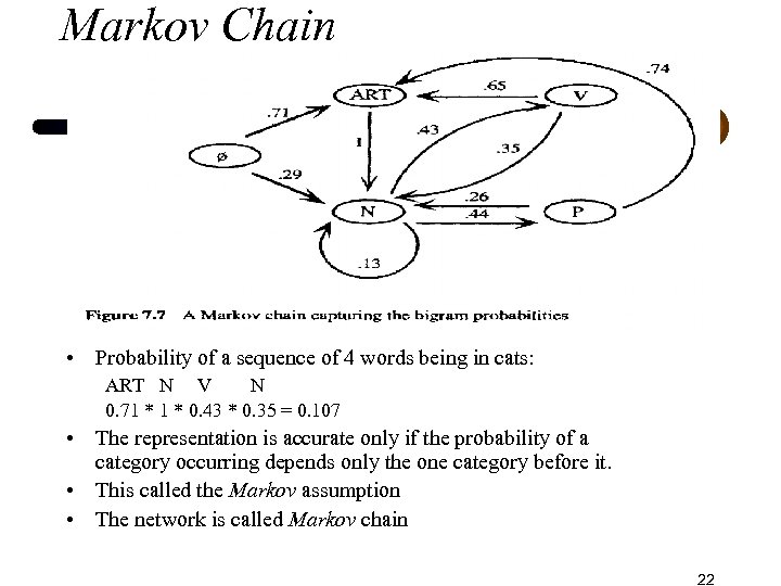 Markov Chain • Probability of a sequence of 4 words being in cats: ART N V N 0. 71 * 0. 43 * 0. 35 = 0. 107 • The representation is accurate only if the probability of a category occurring depends only the one category before it. • This called the Markov assumption • The network is called Markov chain 22
 Hidden Markov Model (HMM) • Markov network can be extended to include the lexical-generation probabilities, too. • Each node could have an output probability for its every possible corresponding output • The output probabilities are exactly the lexicalgeneration probabilities shown in fig 7 -6 • Markov network with output probabilities is called Hidden Markov Model (HMM) 23
 Hidden Markov Model (HMM) • The word hidden indicates that for a specific sequence of words, it is not clear what state the Markov model is in • For instance, the word “flies” could be generated from state N with a probability of 0. 25, or from state V with a probability of 0. 076 • Now, it is not trivial to compute the probability of a sequence of words from the network 24
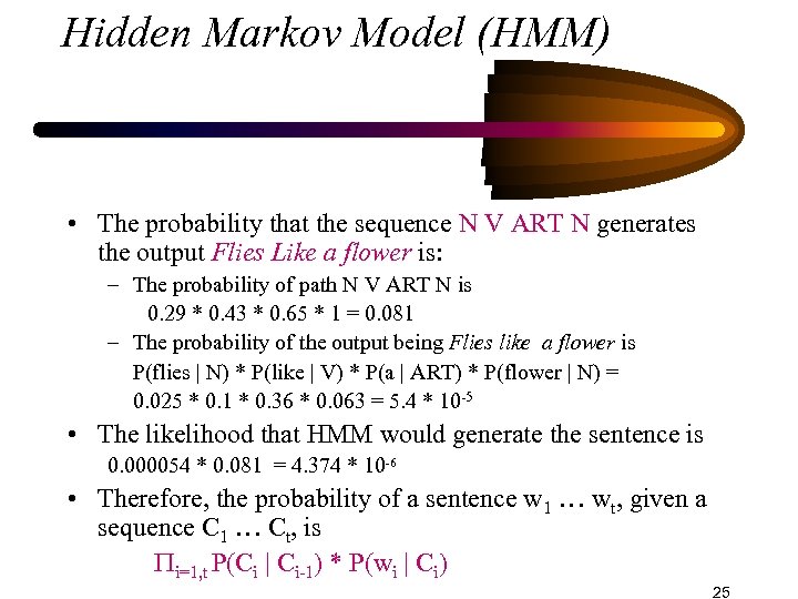 Hidden Markov Model (HMM) • The probability that the sequence N V ART N generates the output Flies Like a flower is: – The probability of path N V ART N is 0. 29 * 0. 43 * 0. 65 * 1 = 0. 081 – The probability of the output being Flies like a flower is P(flies | N) * P(like | V) * P(a | ART) * P(flower | N) = 0. 025 * 0. 1 * 0. 36 * 0. 063 = 5. 4 * 10 -5 • The likelihood that HMM would generate the sentence is 0. 000054 * 0. 081 = 4. 374 * 10 -6 • Therefore, the probability of a sentence w 1 … wt, given a sequence C 1 … Ct, is i=1, t P(Ci | Ci-1) * P(wi | Ci) 25
 Markov Chain 26
 Viterbi Algorithm 27
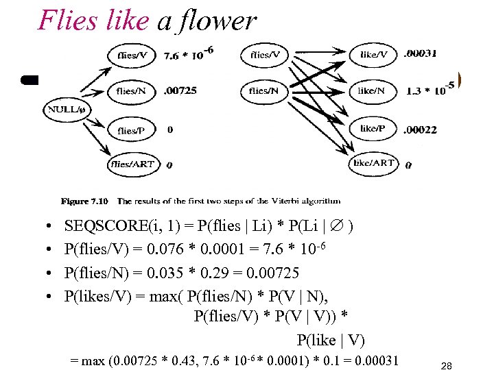 Flies like a flower • • SEQSCORE(i, 1) = P(flies | Li) * P(Li | ) P(flies/V) = 0. 076 * 0. 0001 = 7. 6 * 10 -6 P(flies/N) = 0. 035 * 0. 29 = 0. 00725 P(likes/V) = max( P(flies/N) * P(V | N), P(flies/V) * P(V | V)) * P(like | V) = max (0. 00725 * 0. 43, 7. 6 * 10 -6 * 0. 0001) * 0. 1 = 0. 00031 28
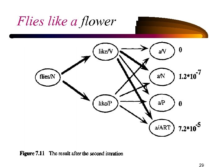 Flies like a flower 29
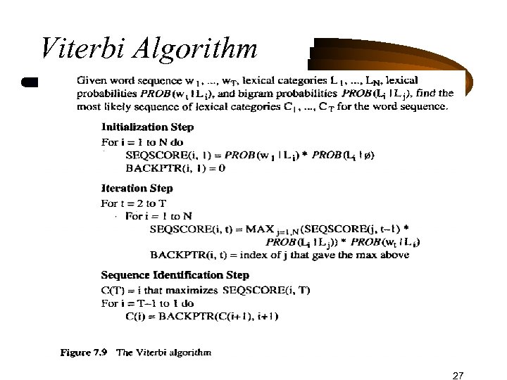
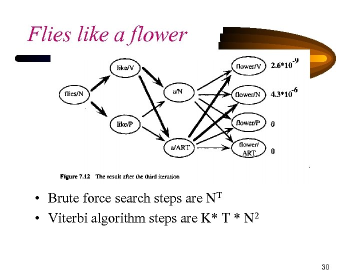 Flies like a flower • Brute force search steps are NT • Viterbi algorithm steps are K* T * N 2 30
 Getting Reliable Statistics (smoothing) • Suppose we have 40 categories • To collect unigrams, at least 40 samples, one for each category, are needed • For bigrams, 1600 samples are needed • For trigerams, 64000 samples are needed • For 4 -grams, 2560000 samples are needed • P(Ci | C … Ci-1) = 1 P(Ci) + 2 P(Ci | Ci-1) + 3 P(Ci | Ci-2 Ci-1) • 1+ 2 + 3 = 1 31
 Statistical Parsing • Corpus-based methods offer new ways to control parsers • We could use statistical methods to identify the common structures of a Language • We can choose the most likely interpretation when a sentence is ambiguous • This might lead to much more efficient parsers that are almost deterministic 32
 Statistical Parsing • • What is the input of an statistical parser? Input is the output of a POS tagging algorithm If POSs are accurate, lexical ambiguity is removed But if tagging is wrong, parser cannot find the correct interpretation, or, may find a valid but implausible interpretation • With %95 accuracy, the chance of correctly tagging a sentence of 8 words is 0. 67, and that of 15 words is 0. 46 33
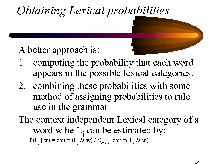 Obtaining Lexical probabilities A better approach is: 1. computing the probability that each word appears in the possible lexical categories. 2. combining these probabilities with some method of assigning probabilities to rule use in the grammar The context independent Lexical category of a word w be Lj can be estimated by: P(Lj | w) = count (Lj & w) / i=1, N count( Li & w) 34
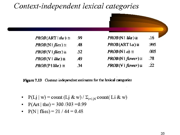 Context-independent lexical categories • P(Lj | w) = count (Lj & w) / i=1, N count( Li & w) • P(Art | the) = 300 /303 =0. 99 • P(N | flies) = 21 / 44 = 0. 48 35
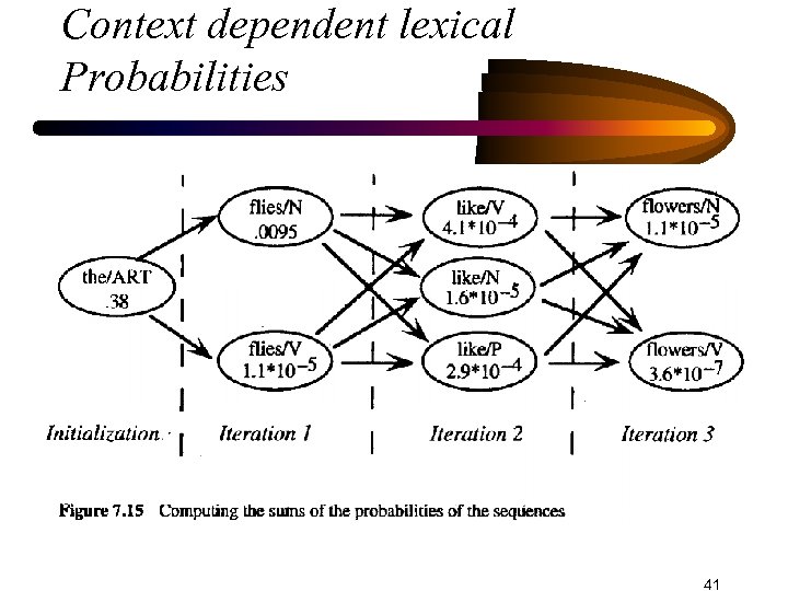
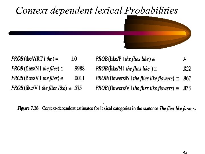
 Context dependent lexical probabilities • A better estimate can be obtained by computing how likely it is that category Li occurs at position t, in all sequences of the input w 1 … wt • Instead of just finding the sequence with the maximum probability, we add up the probabilities of all sequences that end in wt/Li • The probability that flies is a noun in the sentence The flies like flowers is calculated by adding the probability of all sequences that end with flies as a noun 36
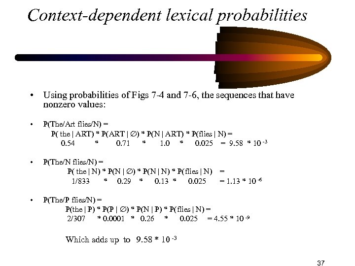 Context-dependent lexical probabilities • Using probabilities of Figs 7 -4 and 7 -6, the sequences that have nonzero values: • P(The/Art flies/N) = P( the | ART) * P(ART | ) * P(N | ART) * P(flies | N) = 0. 54 * 0. 71 * 1. 0 * 0. 025 = 9. 58 * 10 -3 • P(The/N flies/N) = P( the | N) * P(N | N) * P(flies | N) = 1/833 * 0. 29 * 0. 13 * 0. 025 = 1. 13 * 10 -6 • P(The/P flies/N) = P(the | P) * P(P | ) * P(N | P) * P(flies | N) = 2/307 * 0. 0001 * 0. 26 * 0. 025 = 4. 55 * 10 -9 Which adds up to 9. 58 * 10 -3 37
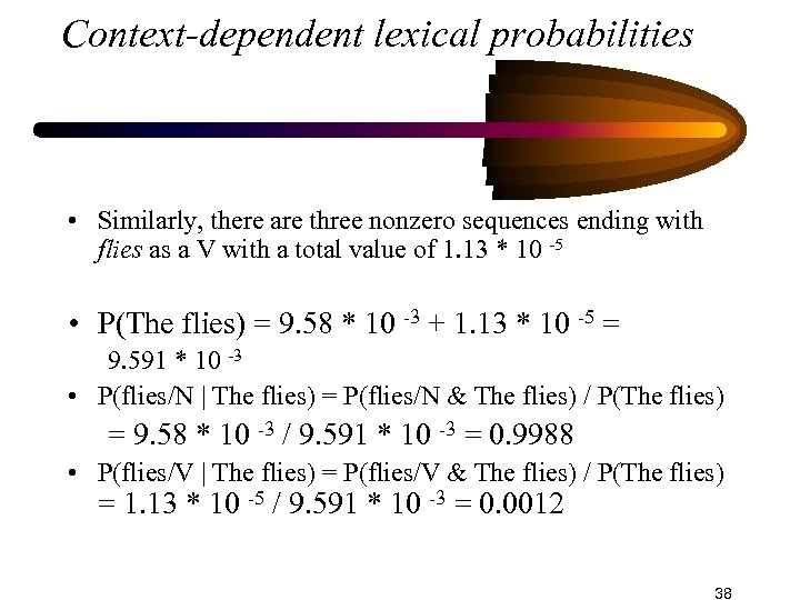 Context-dependent lexical probabilities • Similarly, there are three nonzero sequences ending with flies as a V with a total value of 1. 13 * 10 -5 • P(The flies) = 9. 58 * 10 -3 + 1. 13 * 10 -5 = 9. 591 * 10 -3 • P(flies/N | The flies) = P(flies/N & The flies) / P(The flies) = 9. 58 * 10 -3 / 9. 591 * 10 -3 = 0. 9988 • P(flies/V | The flies) = P(flies/V & The flies) / P(The flies) = 1. 13 * 10 -5 / 9. 591 * 10 -3 = 0. 0012 38
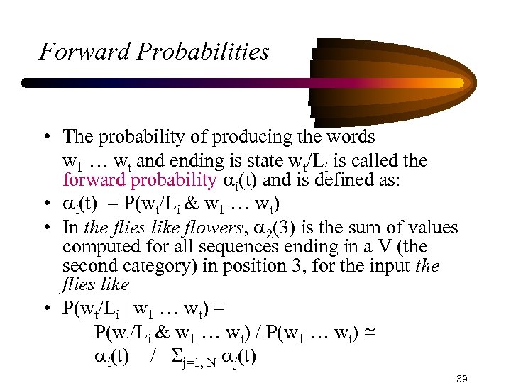 Forward Probabilities • The probability of producing the words w 1 … wt and ending is state wt/Li is called the forward probability i(t) and is defined as: • i(t) = P(wt/Li & w 1 … wt) • In the flies like flowers, 2(3) is the sum of values computed for all sequences ending in a V (the second category) in position 3, for the input the flies like • P(wt/Li | w 1 … wt) = P(wt/Li & w 1 … wt) / P(w 1 … wt) i(t) / j=1, N j(t) 39
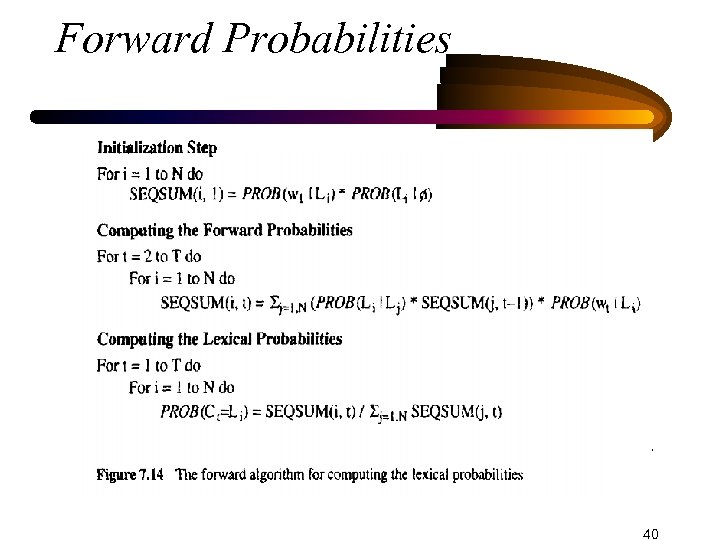 Forward Probabilities 40
 Context dependent lexical Probabilities 41
 Context dependent lexical Probabilities 42
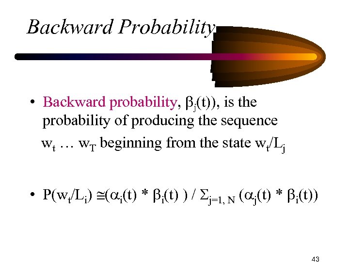 Backward Probability • Backward probability, j(t)), is the probability of producing the sequence wt … w. T beginning from the state wt/Lj • P(wt/Li) ( i(t) * i(t) ) / j=1, N ( j(t) * i(t)) 43
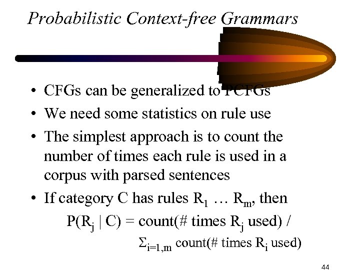 Probabilistic Context-free Grammars • CFGs can be generalized to PCFGs • We need some statistics on rule use • The simplest approach is to count the number of times each rule is used in a corpus with parsed sentences • If category C has rules R 1 … Rm, then P(Rj | C) = count(# times Rj used) / i=1, m count(# times Ri used) 44
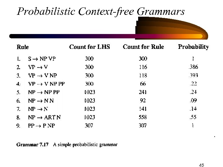 Probabilistic Context-free Grammars 45
 Independence assumption • You can develop algorithm similar to the Veterbi algorithm that finds the most probable parse tree for an input • Certain independence assumptions must be made • The probability of a constituent being derived by a rule Rj is independent of how the constituent is used as a sub constituent • The probabilities of NP rules are the same no matter the NP is the subject, the object of a verb, or the object of a proposition • This assumption is not valid; a subject NP is much more likely to be a pronoun than an object NP 46
 Inside Probability • The probability that a constituent C generates a sequence of words wi, wi+1, …, wj (written as wi, j) is called the inside probability and is denoted as P(wi, j | C) • It is called inside probability because it assigns a probability to the word sequence inside the constituent 47
 Inside Probabilities • How to derive inside probabilities? • For lexical categories, these are the same as lexicalgeneration probabilities • P(flower | N) is the inside probability that the constituent N is realized as the word flower (0. 06 in fig. 7 -6) • Using lexical-generation probabilities, inside probabilities of Non-lexical constituents can be computed 48
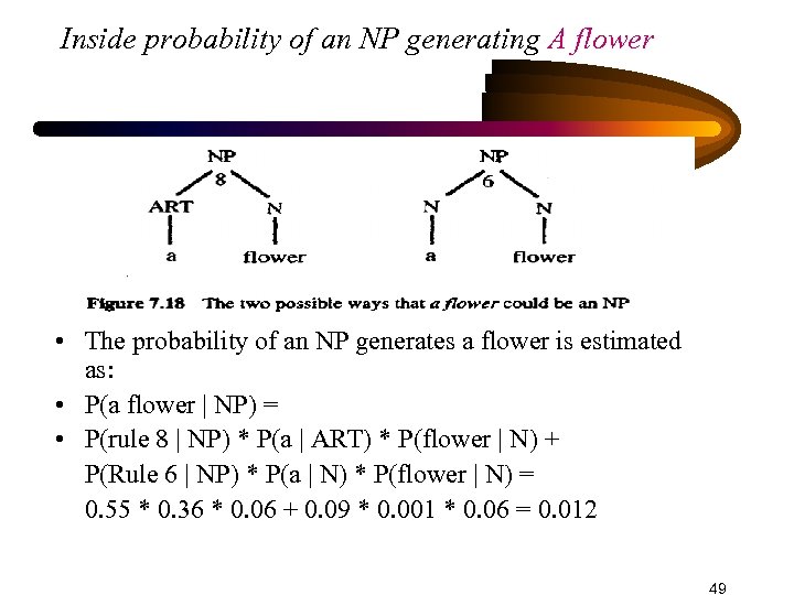 Inside probability of an NP generating A flower • The probability of an NP generates a flower is estimated as: • P(a flower | NP) = • P(rule 8 | NP) * P(a | ART) * P(flower | N) + P(Rule 6 | NP) * P(a | N) * P(flower | N) = 0. 55 * 0. 36 * 0. 06 + 0. 09 * 0. 001 * 0. 06 = 0. 012 49
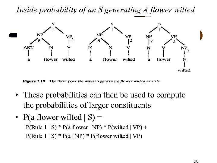 Inside probability of an S generating A flower wilted • These probabilities can then be used to compute the probabilities of larger constituents • P(a flower wilted | S) = P(Rule 1 | S) * P(a flower | NP) * P(wilted | VP) + P(Rule 1 | S) * P(a | NP) * P(flower wilted | VP) 50
 Probabilistic chart parsing • In parsing, we are interested in finding the most likely parse rather than the overall probability of a given sentence. • We can a Chart Parser for this propose • When entering an entry E of category C using rule i with n sub constituents corresponding to entries E 1 … En, then • P(E) = P(Rule i | C) * P(E 1) * … * P(En) • For lexical categories, it is better to use forward probabilities rather than lexical-generation probs. 51
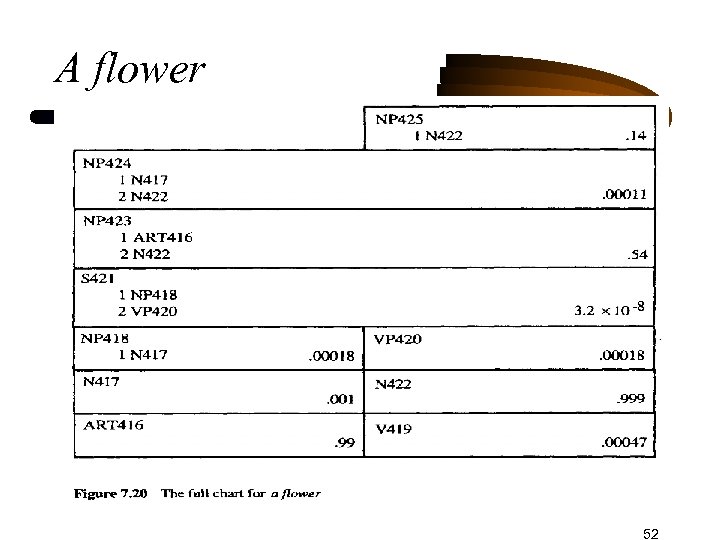 A flower 52
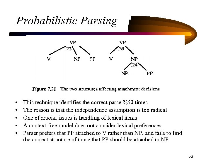 Probabilistic Parsing • • • This technique identifies the correct parse %50 times The reason is that the independence assumption is too radical One of crucial issues is handling of lexical items A context-free model does not consider lexical preferences Parser prefers that PP attached to V rather than NP, and fails to find the correct structure of those that PP should be attached to NP 53
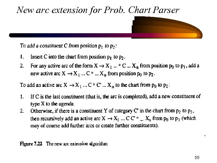
 Best-First Parsing • Exploring higher probability constituents first • Much of the search space, containing lowerrated probabilities is not explored • Chart parser’s Agenda is organized as a priority queue • Arc extension algorithm need to be modified 54
 New arc extension for Prob. Chart Parser 55
 The man put a bird in the house • Best first parser finds the correct parse after generating 65 constituents, • Standard bottom-up parser generates 158 constituents • Standard algorithm generates 106 constituents to find the first answer • So, the best-first parsing is a significant improvement 56
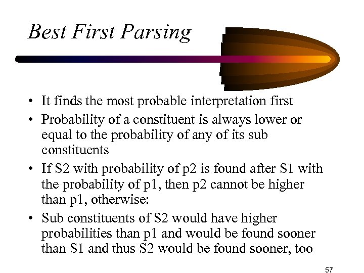 Best First Parsing • It finds the most probable interpretation first • Probability of a constituent is always lower or equal to the probability of any of its sub constituents • If S 2 with probability of p 2 is found after S 1 with the probability of p 1, then p 2 cannot be higher than p 1, otherwise: • Sub constituents of S 2 would have higher probabilities than p 1 and would be found sooner than S 1 and thus S 2 would be found sooner, too 57
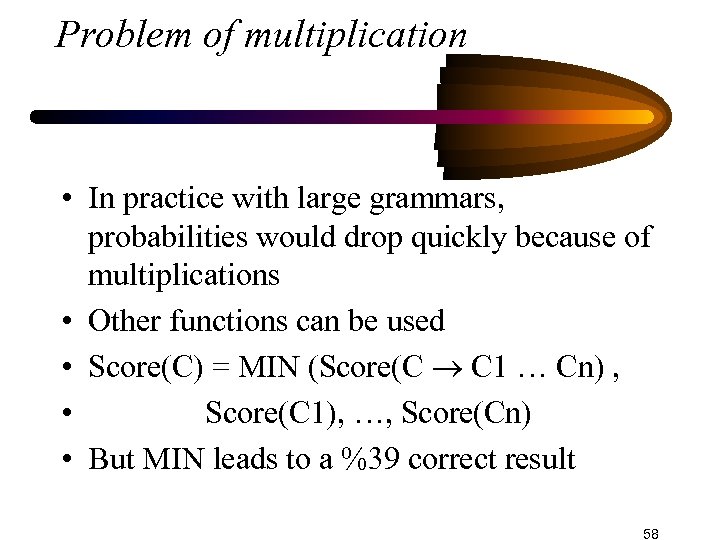 Problem of multiplication • In practice with large grammars, probabilities would drop quickly because of multiplications • Other functions can be used • Score(C) = MIN (Score(C C 1 … Cn) , • Score(C 1), …, Score(Cn) • But MIN leads to a %39 correct result 58
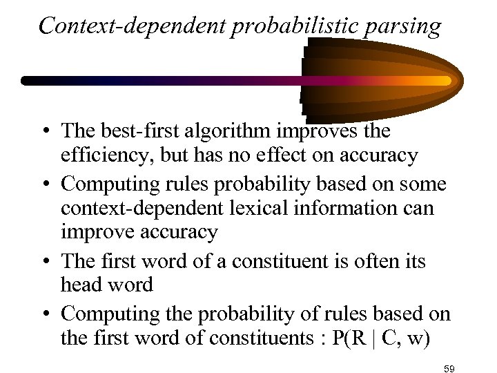 Context-dependent probabilistic parsing • The best-first algorithm improves the efficiency, but has no effect on accuracy • Computing rules probability based on some context-dependent lexical information can improve accuracy • The first word of a constituent is often its head word • Computing the probability of rules based on the first word of constituents : P(R | C, w) 59
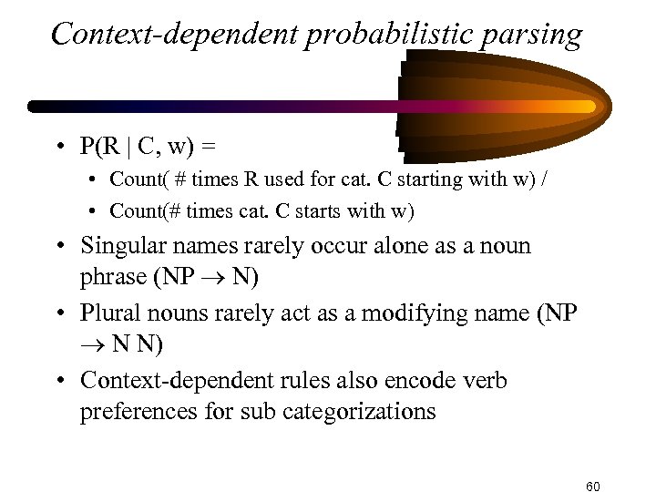 Context-dependent probabilistic parsing • P(R | C, w) = • Count( # times R used for cat. C starting with w) / • Count(# times cat. C starts with w) • Singular names rarely occur alone as a noun phrase (NP N) • Plural nouns rarely act as a modifying name (NP N N) • Context-dependent rules also encode verb preferences for sub categorizations 60
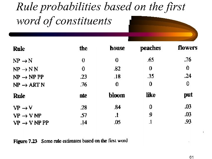 Rule probabilities based on the first word of constituents 61
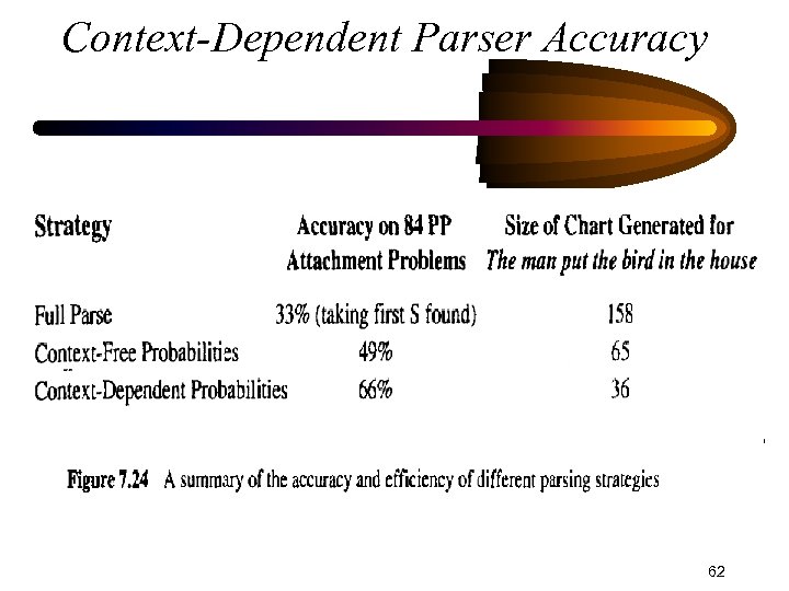 Context-Dependent Parser Accuracy 62
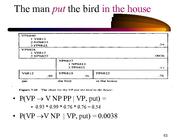 The man put the bird in the house • P(VP V NP PP | VP, put) = • 0. 93 * 0. 99 * 0. 76 = 0. 54 • P(VP V NP | VP, put) = 0. 0038 63
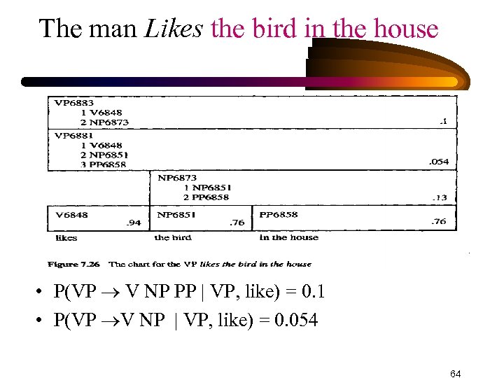 The man Likes the bird in the house • P(VP V NP PP | VP, like) = 0. 1 • P(VP V NP | VP, like) = 0. 054 64
 Context-dependent rules • The accuracy of the parser is still %66 • Make the rule probabilities relative to larger fragment of input (bigram, trigram, …) • Using other important words, such as prepositions • The more selective the lexical categories, the more predictive the estimates can be (provided that there is enough data) • Other closed class words such as articles, quantifiers, conjunctions can also be used (i. e. , treated individually) • But what about open class words such as verbs and nouns (cluster similar words) 65
 Handling Unknown Words • An unknown word will disrupt the parse • Suppose we have a trigram model of data • If w 3 in the sequence of words w 1 w 2 w 3 is unknown, and if w 1 and w 2 are of categories C 1 and C 2 • Pick the category C for w 3 such that P(C | C 1 C 2) is maximized. • For instance, if C 2 is ART, then C will probably be a NOUN (or an ADJECTIVE) • Morphology can also help • Unknown words ending with –ing are likely a VERB, and those ending with –ly are likely an ADVERB 66


