6643eca03f9f4b0be127e9bf60f93e9f.ppt
- Количество слайдов: 56
 Statistical Machine Translation Part II: Word Alignments and EM Alexander Fraser CIS, LMU München 2015. 10. 27 WPCom 1: WSD and MT
 Administravia • It looks like we will start with Referats around the middle of November – I will propose some literature topics and some project topics next time • I need to end class early today, the lecture will go to about 17: 10
 Where we have been • Parallel corpora • Sentence alignment • Overview of statistical machine translation – Start with parallel corpus – Sentence align it – Build SMT system • Parameter estimation – Given new text, decode • Human evaluation & BLEU 3
 Where we are going • Start with sentence aligned parallel corpus • Estimate parameters – Word alignment – Build phrase-based SMT model • Given new text, translate it! – Decoding 4
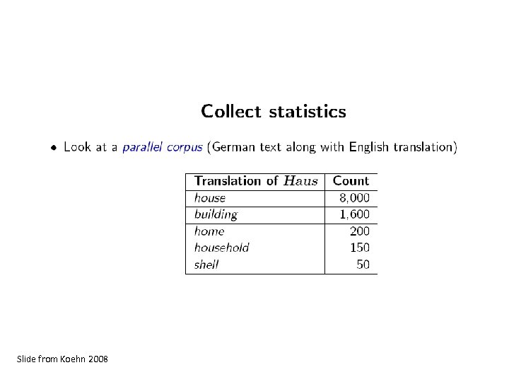
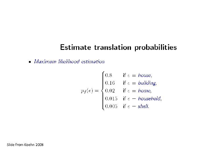
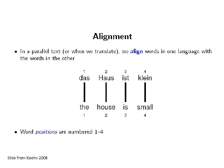
 Word Alignments • Recall that we build translation models from word-aligned parallel sentences – The statistics involved in state of the art SMT decoding models are simple – Just count translations in the word-aligned parallel sentences • But what is a word alignment, and how do we obtain it? 5
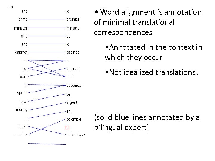 • Word alignment is annotation of minimal translational correspondences • Annotated in the context in which they occur • Not idealized translations! (solid blue lines annotated by a bilingual expert)
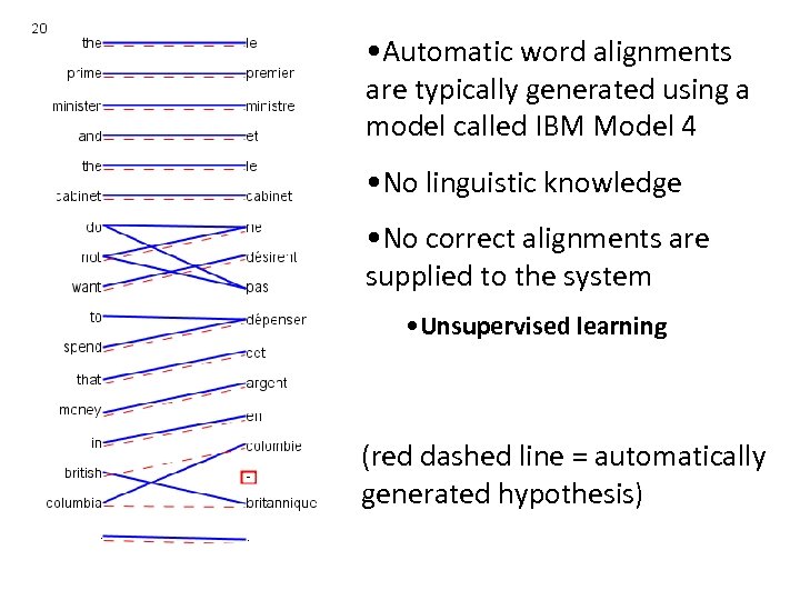 • Automatic word alignments are typically generated using a model called IBM Model 4 • No linguistic knowledge • No correct alignments are supplied to the system • Unsupervised learning (red dashed line = automatically generated hypothesis)
 Uses of Word Alignment • Multilingual – – – Machine Translation Cross-Lingual Information Retrieval Translingual Coding (Annotation Projection) Document/Sentence Alignment Extraction of Parallel Sentences from Comparable Corpora • Monolingual – – Paraphrasing Query Expansion for Monolingual Information Retrieval Summarization Grammar Induction 8
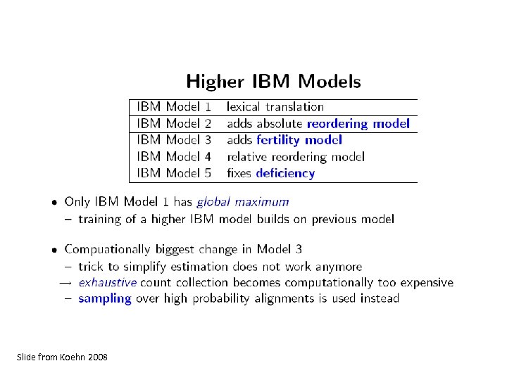
 Outline • Measuring alignment quality • Types of alignments • IBM Model 1 – Training IBM Model 1 with Expectation Maximization • IBM Models 3 and 4 – Approximate Expectation Maximization • Heuristics for high quality alignments from the IBM models
 How to measure alignment quality? • If we want to compare two word alignment algorithms, we can generate a word alignment with each algorithm for fixed training data – Then build an SMT system from each alignment – Compare performance of the SMT systems using BLEU • But this is slow, building SMT systems can take days of computation – Question: Can we have an automatic metric like BLEU, but for alignment? – Answer: yes, by comparing with gold standard alignments 10
 Measuring Precision and Recall • Precision is percentage of links in hypothesis that are correct – If we hypothesize there are no links, have 100% precision • Recall is percentage of correct links we hypothesized – If we hypothesize all possible links, have 100% recall 11
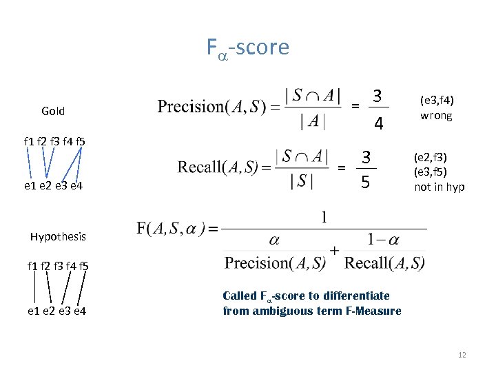 F -score Gold f 1 f 2 f 3 f 4 f 5 e 1 e 2 e 3 e 4 = 3 4 3 = 5 (e 3, f 4) wrong (e 2, f 3) (e 3, f 5) not in hyp Hypothesis f 1 f 2 f 3 f 4 f 5 e 1 e 2 e 3 e 4 Called F -score to differentiate from ambiguous term F-Measure 12
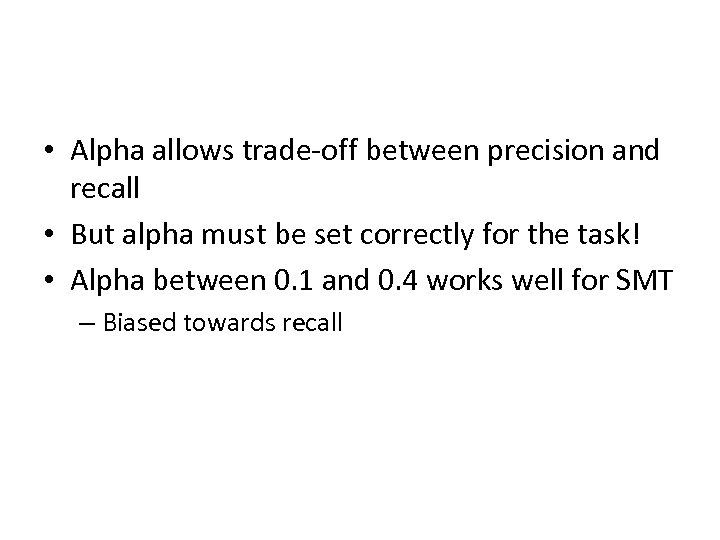 • Alpha allows trade-off between precision and recall • But alpha must be set correctly for the task! • Alpha between 0. 1 and 0. 4 works well for SMT – Biased towards recall
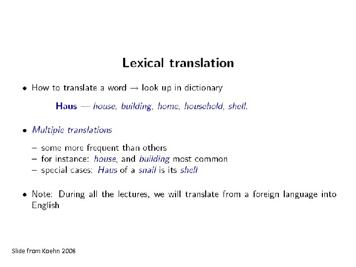 Slide from Koehn 2008
 Slide from Koehn 2008
 Slide from Koehn 2008
 Slide from Koehn 2008
 Slide from Koehn 2008
 Slide from Koehn 2008
 Slide from Koehn 2008
 Slide from Koehn 2008
 Slide from Koehn 2008
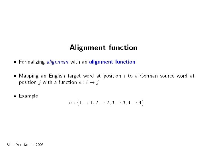
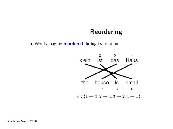
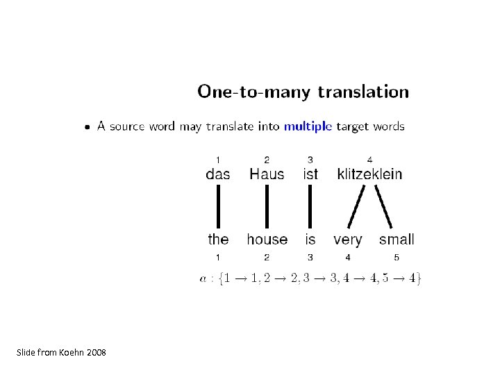
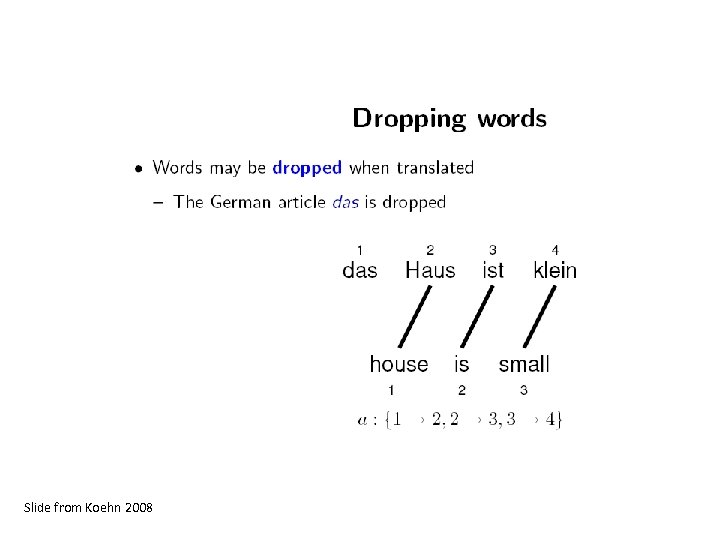
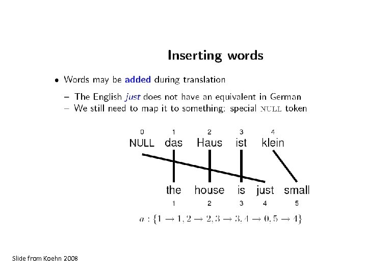
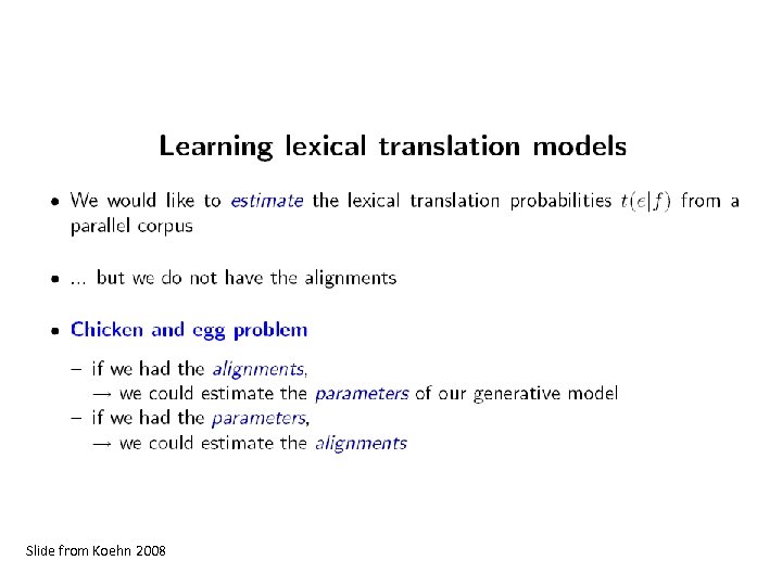
 Last word on alignment functions • Alignments functions are nice because they are a simple representation of the alignment graph • However, they are strangely asymmetric – There is a NULL word on the German side (to explain where unlinked English words came from) – But no NULL word on the English side (some German words simply don’t generate anything) – Very important: alignment functions do not allow us to represent two or more German words being linked to one English word! • But we will deal with this later… • Now let’s talk about models
 Generative Word Alignment Models • We observe a pair of parallel sentences (e, f) • We would like to know the highest probability alignment a for (e, f) • Generative models are models that follow a series of steps – We will pretend that e has been generated from f – The sequence of steps to do this is encoded in the alignment a – A generative model associates a probability p(e, a|f) to each alignment • In words, this is the probability of generating the alignment a and the English sentence e, given the foreign sentence f
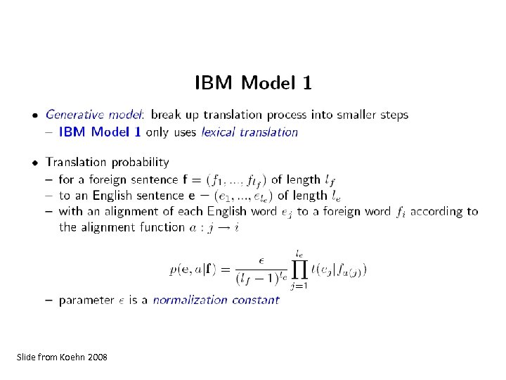
 IBM Model 1 A simple generative model, start with: – foreign sentence f – a lexical mapping distribution t(English. Word|Foreign. Word) How to generate an English sentence e from f: 1. Pick a length for the English sentence at random 2. Pick an alignment function at random 3. For each English position generate an English word by looking up the aligned Foreign. Word in the alignment function, and choose an English word using t
 Slide from Koehn 2008
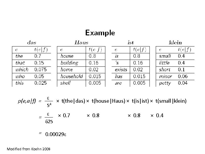 p(e, a|f) = Є 54 625 × t(the|das) × t(house|Haus) × t(is|ist) × t(small|klein) × 0. 7 = 0. 00029Є Modified from Koehn 2008 × 0. 4
 Slide from Koehn 2008
 Slide from Koehn 2008
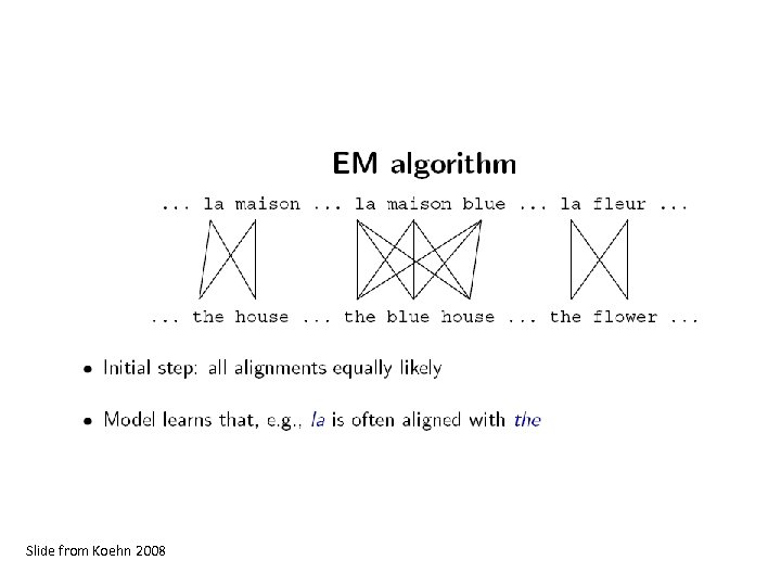
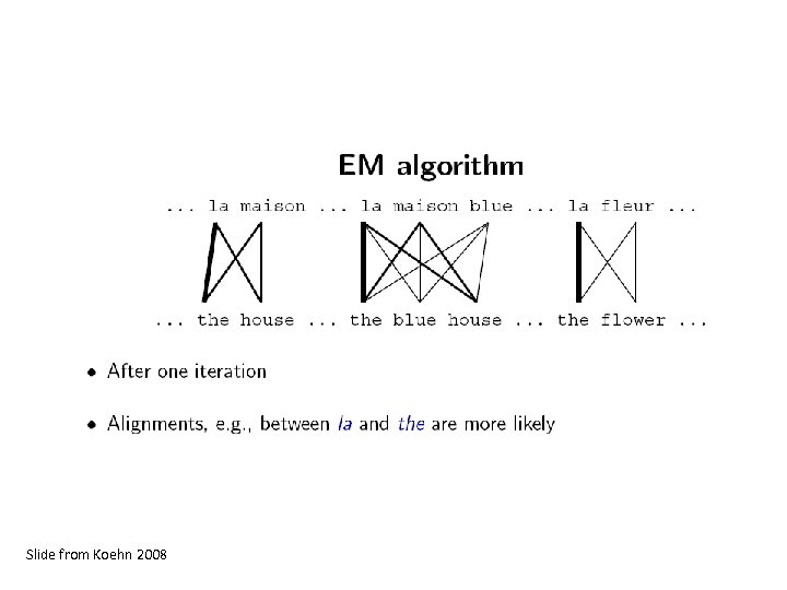
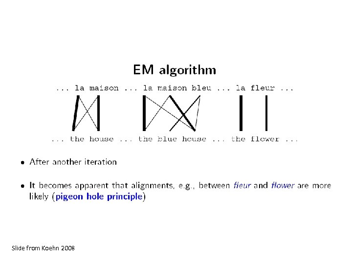
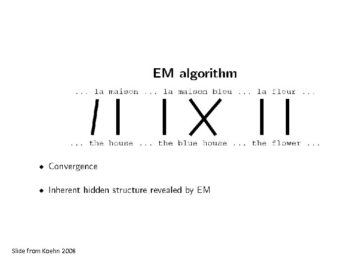
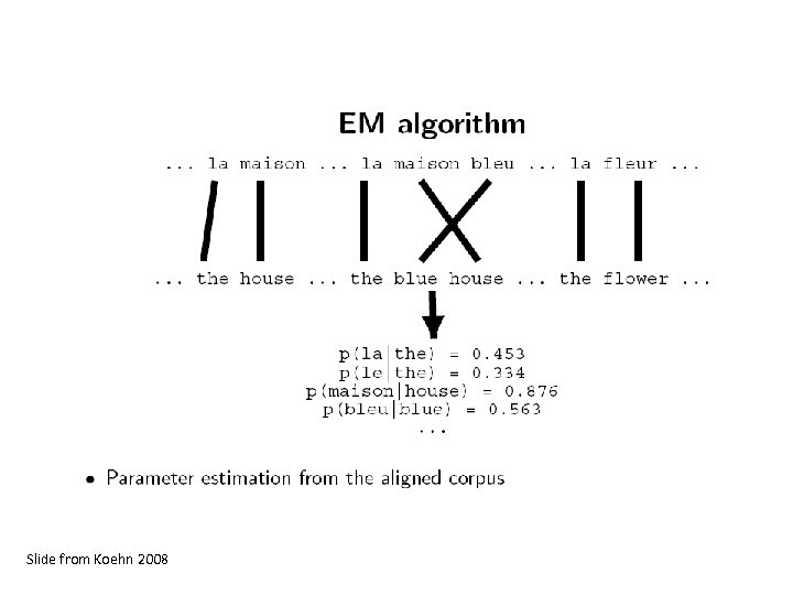
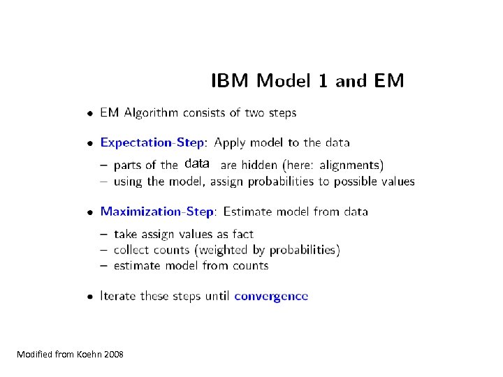
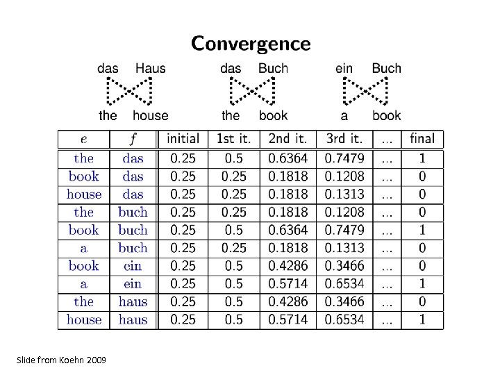
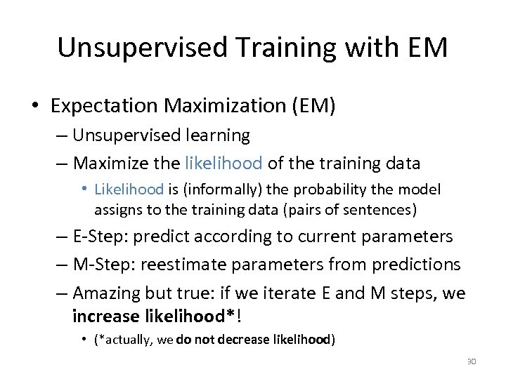 Unsupervised Training with EM • Expectation Maximization (EM) – Unsupervised learning – Maximize the likelihood of the training data • Likelihood is (informally) the probability the model assigns to the training data (pairs of sentences) – E-Step: predict according to current parameters – M-Step: reestimate parameters from predictions – Amazing but true: if we iterate E and M steps, we increase likelihood*! • (*actually, we do not decrease likelihood) 30
 Slide from Koehn 2008
 Slide from Koehn 2008
 Slide from Koehn 2008
 Slide from Koehn 2008
 Slide from Koehn 2008
 data Modified from Koehn 2008
 Slide from Koehn 2008
 We will work out an example for the sentence pair: la maison the house in a few slides, but first, let’s discuss EM further…
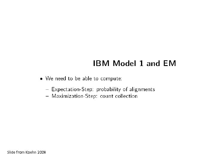
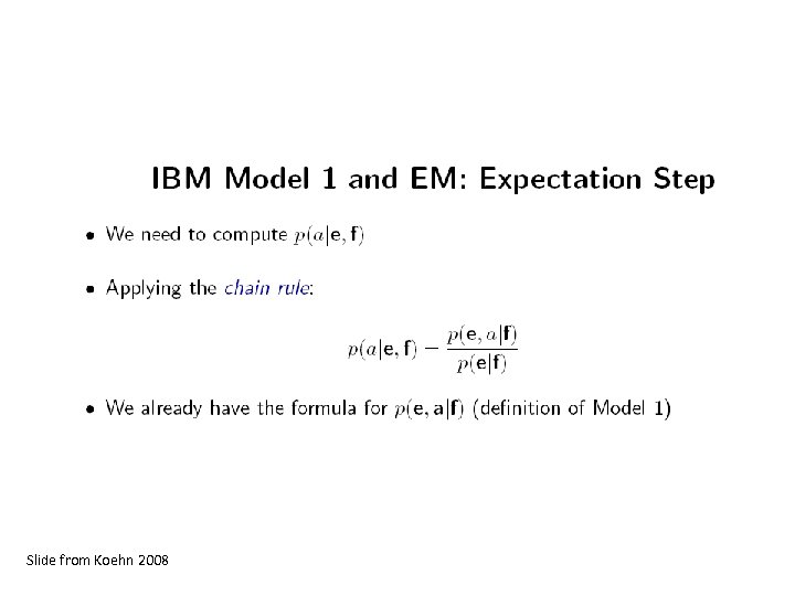
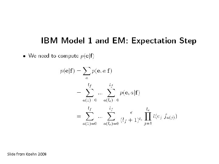
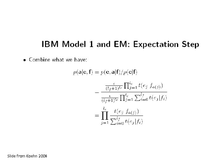
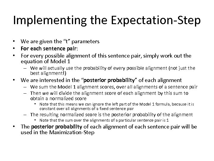 Implementing the Expectation-Step • We are given the “t” parameters • For each sentence pair: • For every possible alignment of this sentence pair, simply work out the equation of Model 1 – We will actually use the probability of every possible alignment (not just the best alignment!) • We are interested in the “posterior probability” of each alignment – We sum the Model 1 alignment scores, over all alignments of a sentence pair – Then we will divide the alignment score of each alignment by this sum to obtain a normalized score • Note that this means we can ignore the left part of the Model 1 formula, because it is constant over all alignments of a fixed sentence pair – The resulting normalized score is the posterior probability of the alignment • Note that the sum over the alignments of a particular sentence pair is 1 • The posterior probability of each alignment of each sentence pair will be used in the Maximization-Step
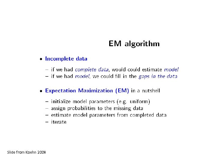
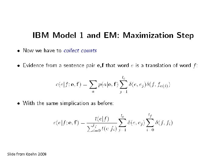
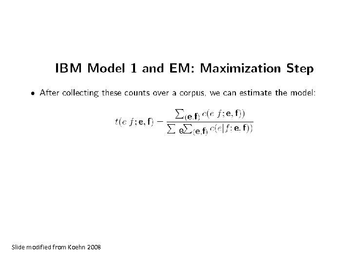
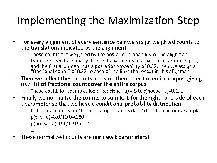 Implementing the Maximization-Step • For every alignment of every sentence pair we assign weighted counts to the translations indicated by the alignment – These counts are weighted by the posterior probability of the alignment – Example: if we have many different alignments of a particular sentence pair, and the first alignment has a posterior probability of 0. 32, then we assign a “fractional count” of 0. 32 to each of the links that occur in this alignment • Then we collect these counts and sum them over the entire corpus, giving us a list of fractional counts over the entire corpus – These could, for example, look like: c(the|la) = 8. 0, c(house|la)=0. 1, … • Finally we normalize the counts to sum to 1 for the right hand side of each t parameter so that we have a conditional probability distribution – – If the total counts for “la” on the right hand side = 10. 0, then, in our example: p(the|la)=8. 0/10. 0=0. 80 p(house|la)=0. 1/10. 0=0. 01 … • These normalized counts are our new t parameters!
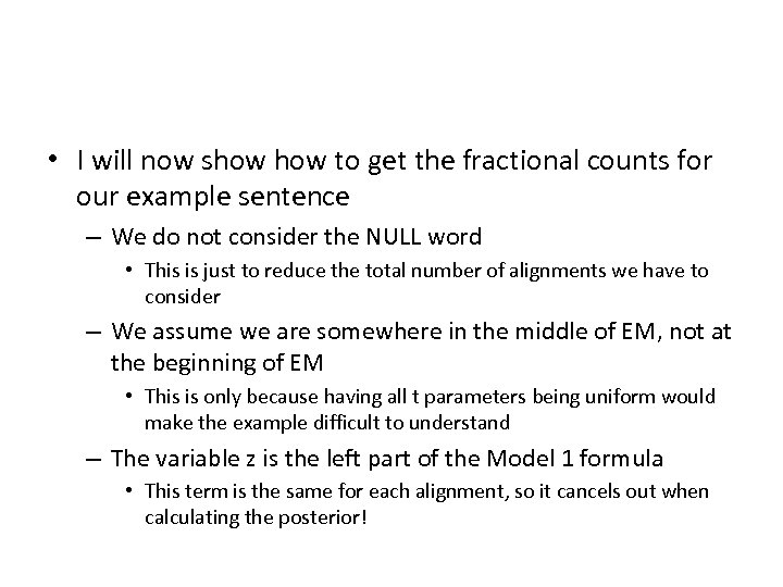 • I will now show to get the fractional counts for our example sentence – We do not consider the NULL word • This is just to reduce the total number of alignments we have to consider – We assume we are somewhere in the middle of EM, not at the beginning of EM • This is only because having all t parameters being uniform would make the example difficult to understand – The variable z is the left part of the Model 1 formula • This term is the same for each alignment, so it cancels out when calculating the posterior!
 Slide from Koehn 2008
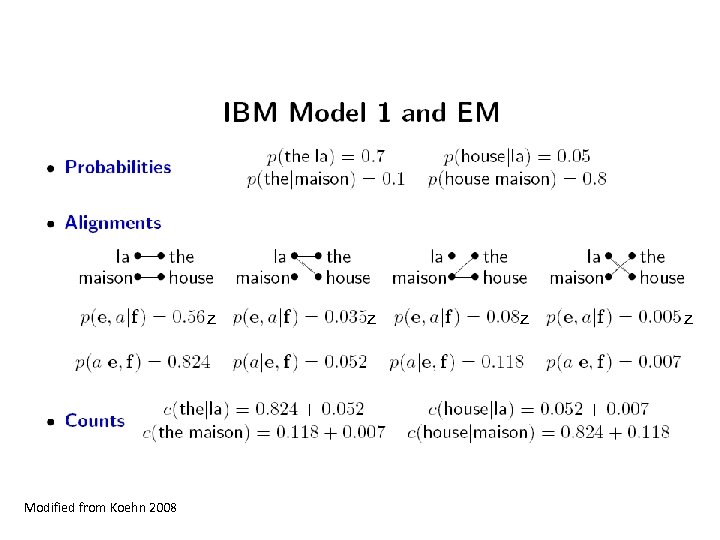 z Modified from Koehn 2008 z z z
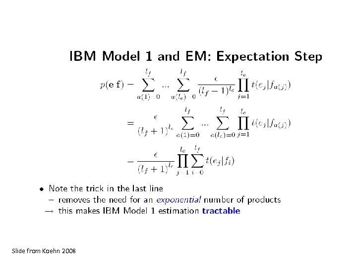
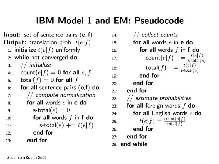
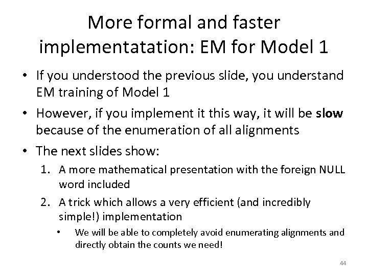 More formal and faster implementatation: EM for Model 1 • If you understood the previous slide, you understand EM training of Model 1 • However, if you implement it this way, it will be slow because of the enumeration of all alignments • The next slides show: 1. A more mathematical presentation with the foreign NULL word included 2. A trick which allows a very efficient (and incredibly simple!) implementation • We will be able to completely avoid enumerating alignments and directly obtain the counts we need! 44
 Slide from Koehn 2008
 Slide from Koehn 2008
 Slide from Koehn 2008
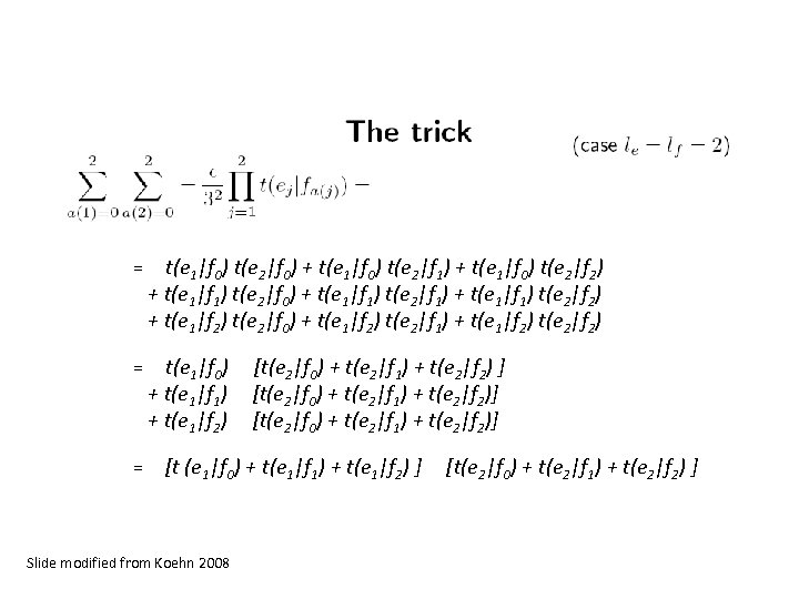 = t(e 1|f 0) t(e 2|f 0) + t(e 1|f 0) t(e 2|f 1) + t(e 1|f 0) t(e 2|f 2) + t(e 1|f 1) t(e 2|f 0) + t(e 1|f 1) t(e 2|f 1) + t(e 1|f 1) t(e 2|f 2) + t(e 1|f 2) t(e 2|f 0) + t(e 1|f 2) t(e 2|f 1) + t(e 1|f 2) t(e 2|f 2) = t(e 1|f 0) + t(e 1|f 1) + t(e 1|f 2) = [t(e 2|f 0) + t(e 2|f 1) + t(e 2|f 2) ] [t(e 2|f 0) + t(e 2|f 1) + t(e 2|f 2)] [t (e 1|f 0) + t(e 1|f 1) + t(e 1|f 2) ] Slide modified from Koehn 2008 [t(e 2|f 0) + t(e 2|f 1) + t(e 2|f 2) ]
 Slide from Koehn 2008
 Collecting Counts • We now have to collect counts from each sentence pair e , f for each word pair e and f • The formula for fixed words e and f is on the next slide • We first need the definition of the Kronecker delta function: δ(a, b) = 1 if a=b 0 otherwise
 Slide from Koehn 2008
 e Slide modified from Koehn 2008
 Slide from Koehn 2009
 Slide from Koehn 2009
 Slide from Koehn 2008
 • Thank you for your attention! 57


