STAT6202 Chapter 2 2012/2013 1 CHAPTER 2 Describing

STAT6202 Chapter 2 2012/2013 1 CHAPTER 2 Describing bivariate data NOTATION SCATTER PLOT SIMPLE LINEAR REGRESSION What is it? Least squares estimation Watch out! Log transformation and regression A practical approach SAMPLE CORRELATION COEFFICIENT RANK CORRELATION COEFICIENT

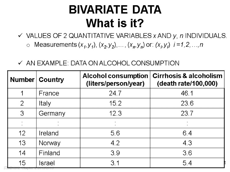
STAT6202 Chapter 2 2012/2013 2 BIVARIATE DATA What is it? VALUES OF 2 QUANTITATIVE VARIABLES x AND y, n INDIVIDUALS. o Measurements (x1,y1), (x2,y2),…, (xn,yn) or: (xi,yi) i =1,2,…,n AN EXAMPLE: DATA ON ALCOHOL CONSUMPTION

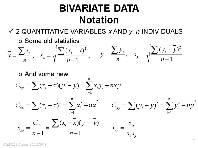
STAT6202 Chapter 2 2012/2013 3 BIVARIATE DATA Notation 2 QUANTITATIVE VARIABLES x AND y, n INDIVIDUALS Some old statistics And some new

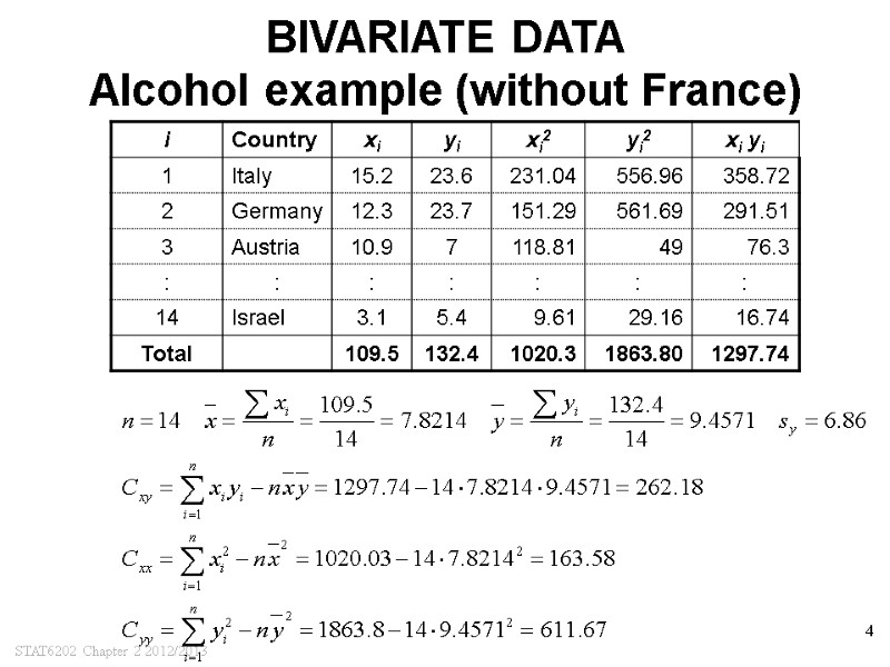
STAT6202 Chapter 2 2012/2013 4 BIVARIATE DATA Alcohol example (without France)

STAT6202 Chapter 2 2012/2013 5 CHAPTER 2 Describing bivariate data NOTATION SCATTER PLOT SIMPLE LINEAR REGRESSION What is it? Least squares estimation Watch out! Log transformation and regression A practical approach SAMPLE CORRELATION COEFFICIENT RANK CORRELATION COEFICIENT

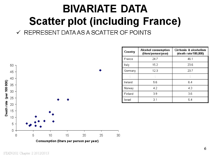
STAT6202 Chapter 2 2012/2013 6 BIVARIATE DATA Scatter plot (including France) REPRESENT DATA AS A SCATTER OF POINTS

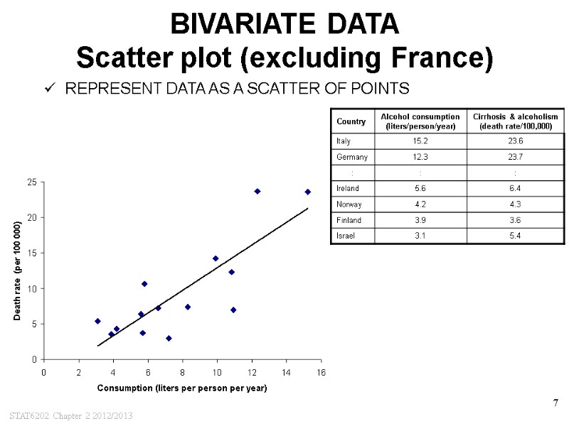
STAT6202 Chapter 2 2012/2013 7 BIVARIATE DATA Scatter plot (excluding France) REPRESENT DATA AS A SCATTER OF POINTS

STAT6202 Chapter 2 2012/2013 8 CHAPTER 2 Describing bivariate data NOTATION SCATTER PLOT SIMPLE LINEAR REGRESSION What is it? Least squares estimation Watch out! Log transformation and regression A practical approach SAMPLE CORRELATION COEFFICIENT RANK CORRELATION COEFICIENT

STAT6202 Chapter 2 2012/2013 9 REGRESSION What is it? It’s everywhere! TRYING TO PREDICT (/EXPLAIN) ONE VARIABLE AS A FUNCTION OF ANOTHER ONE Or multiple other ones ONE OF THE MOST OFTEN USED STATISTICAL TOOLS REGRESSION CAN BE VERY POWERFUL AND COMPLEX WE WILL LOOK AT THE MOST BASIC Simple linear regression: Linear relationship between two variables

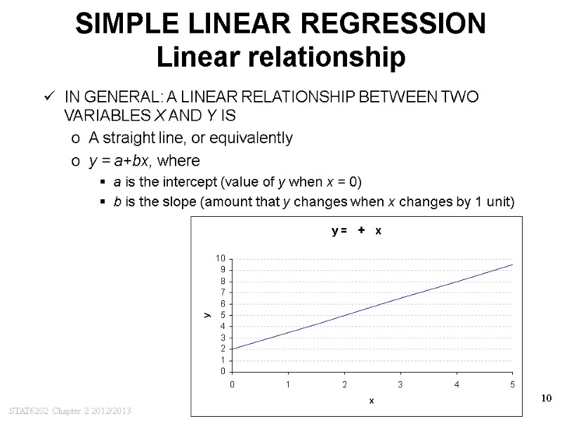
STAT6202 Chapter 2 2012/2013 10 SIMPLE LINEAR REGRESSION Linear relationship IN GENERAL: A LINEAR RELATIONSHIP BETWEEN TWO VARIABLES X AND Y IS A straight line, or equivalently y = a+bx, where a is the intercept (value of y when x = 0) b is the slope (amount that y changes when x changes by 1 unit)

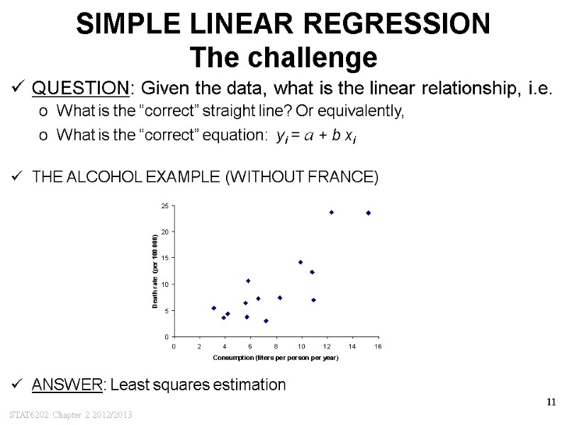
STAT6202 Chapter 2 2012/2013 11 SIMPLE LINEAR REGRESSION The challenge QUESTION: Given the data, what is the linear relationship, i.e. What is the “correct” straight line? Or equivalently, What is the “correct” equation: yi = a + b xi THE ALCOHOL EXAMPLE (WITHOUT FRANCE) ANSWER: Least squares estimation

STAT6202 Chapter 2 2012/2013 12 CHAPTER 2 Describing bivariate data NOTATION SCATTER PLOT SIMPLE LINEAR REGRESSION What is it? Least squares estimation Watch out! Log transformation and regression A practical approach SAMPLE CORRELATION COEFFICIENT RANK CORRELATION COEFICIENT

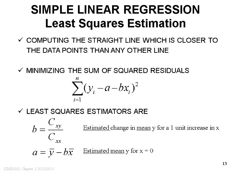
STAT6202 Chapter 2 2012/2013 13 SIMPLE LINEAR REGRESSION Least Squares Estimation COMPUTING THE STRAIGHT LINE WHICH IS CLOSER TO THE DATA POINTS THAN ANY OTHER LINE MINIMIZING THE SUM OF SQUARED RESIDUALS Estimated change in mean y for a 1 unit increase in x Estimated mean y for x = 0 LEAST SQUARES ESTIMATORS ARE

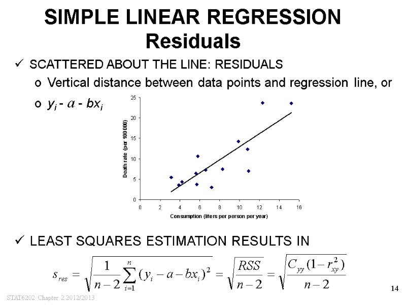
STAT6202 Chapter 2 2012/2013 14 SIMPLE LINEAR REGRESSION Residuals SCATTERED ABOUT THE LINE: RESIDUALS Vertical distance between data points and regression line, or yi - a - bxi LEAST SQUARES ESTIMATION RESULTS IN

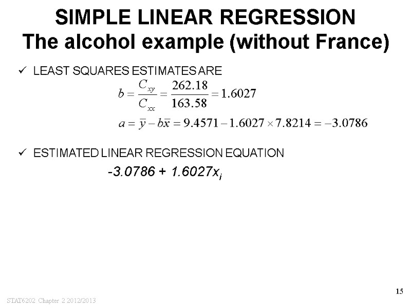
STAT6202 Chapter 2 2012/2013 15 SIMPLE LINEAR REGRESSION The alcohol example (without France) LEAST SQUARES ESTIMATES ARE ESTIMATED LINEAR REGRESSION EQUATION -3.0786 + 1.6027xi

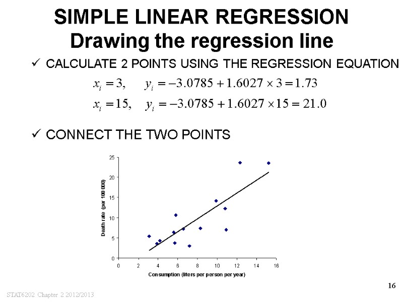
STAT6202 Chapter 2 2012/2013 16 SIMPLE LINEAR REGRESSION Drawing the regression line CALCULATE 2 POINTS USING THE REGRESSION EQUATION CONNECT THE TWO POINTS

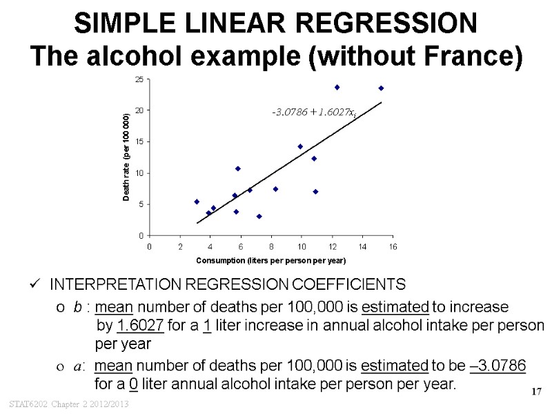
STAT6202 Chapter 2 2012/2013 17 SIMPLE LINEAR REGRESSION The alcohol example (without France) INTERPRETATION REGRESSION COEFFICIENTS b : mean number of deaths per 100,000 is estimated to increase by 1.6027 for a 1 liter increase in annual alcohol intake per person per year a: mean number of deaths per 100,000 is estimated to be –3.0786 for a 0 liter annual alcohol intake per person per year. -3.0786 + 1.6027xi

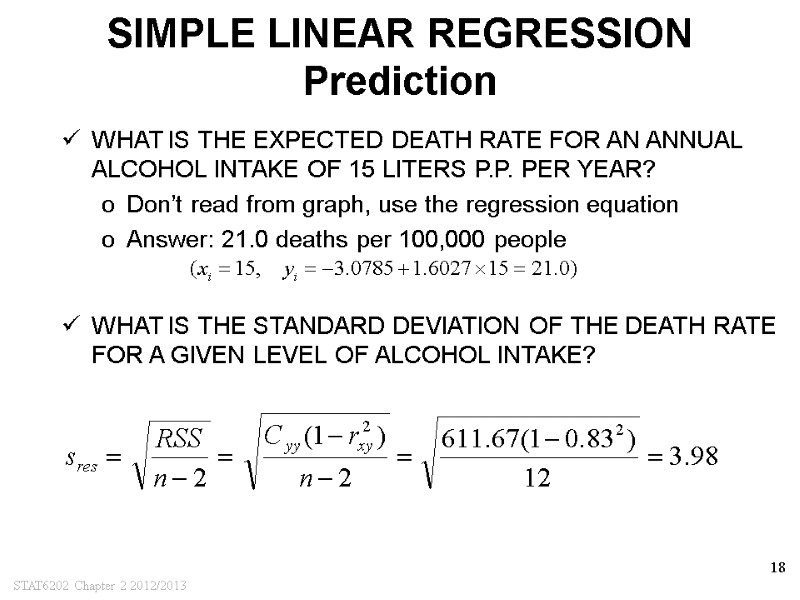
STAT6202 Chapter 2 2012/2013 18 SIMPLE LINEAR REGRESSION Prediction WHAT IS THE EXPECTED DEATH RATE FOR AN ANNUAL ALCOHOL INTAKE OF 15 LITERS P.P. PER YEAR? Don’t read from graph, use the regression equation Answer: 21.0 deaths per 100,000 people WHAT IS THE STANDARD DEVIATION OF THE DEATH RATE FOR A GIVEN LEVEL OF ALCOHOL INTAKE?

STAT6202 Chapter 2 2012/2013 19 CHAPTER 2 Describing bivariate data NOTATION SCATTER PLOT SIMPLE LINEAR REGRESSION What is it? Least squares estimation Watch out! Log transformation and regression A practical approach SAMPLE CORRELATION COEFFICIENT RANK CORRELATION COEFICIENT

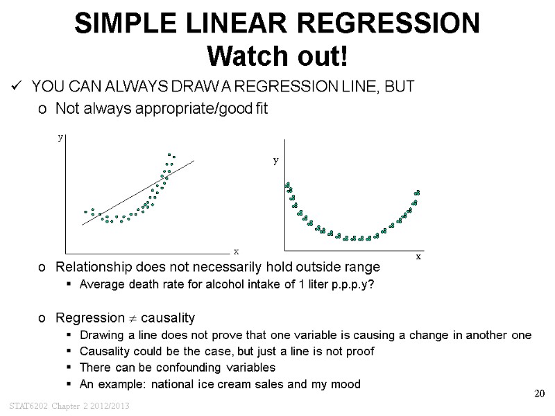
STAT6202 Chapter 2 2012/2013 20 SIMPLE LINEAR REGRESSION Watch out! YOU CAN ALWAYS DRAW A REGRESSION LINE, BUT Not always appropriate/good fit Relationship does not necessarily hold outside range Average death rate for alcohol intake of 1 liter p.p.p.y? Regression  causality Drawing a line does not prove that one variable is causing a change in another one Causality could be the case, but just a line is not proof There can be confounding variables An example: national ice cream sales and my mood

STAT6202 Chapter 2 2012/2013 21 CHAPTER 2 Describing bivariate data NOTATION SCATTER PLOT SIMPLE LINEAR REGRESSION What is it? Least squares estimation Watch out! Log transformation and regression A practical approach SAMPLE CORRELATION COEFFICIENT RANK CORRELATION COEFICIENT

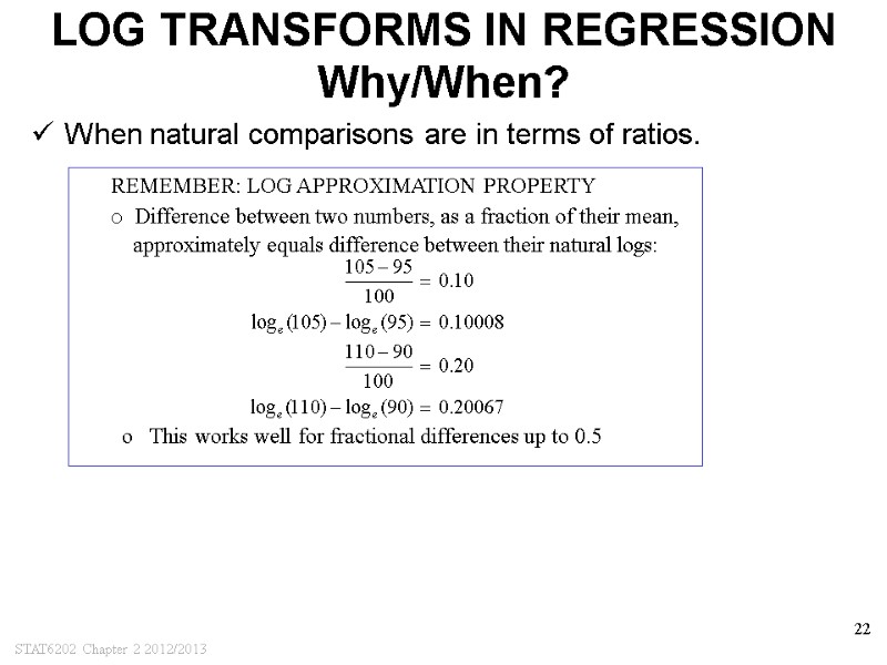
STAT6202 Chapter 2 2012/2013 22 LOG TRANSFORMS IN REGRESSION Why/When? When natural comparisons are in terms of ratios. REMEMBER: LOG APPROXIMATION PROPERTY o Difference between two numbers, as a fraction of their mean, approximately equals difference between their natural logs: This works well for fractional differences up to 0.5

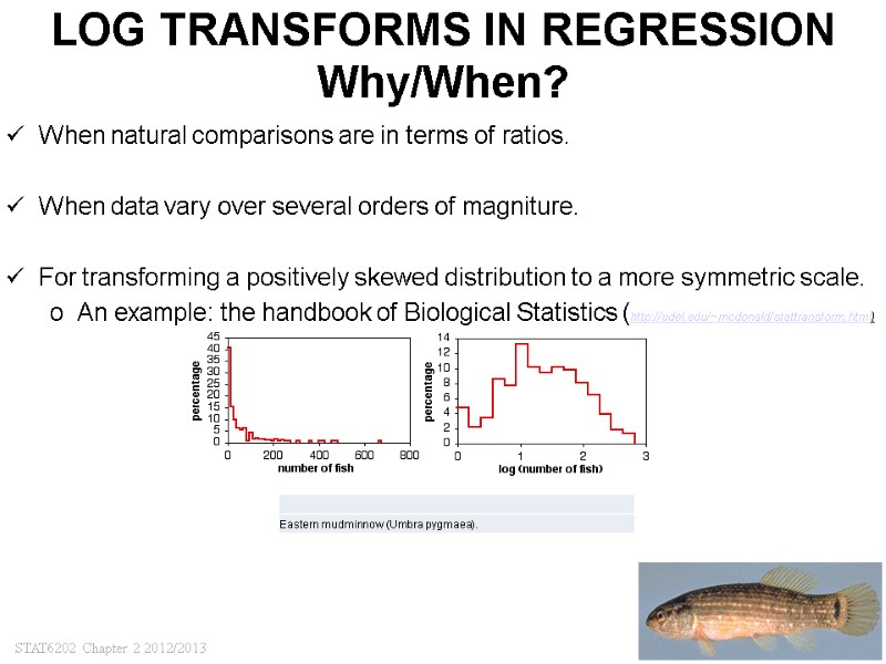
STAT6202 Chapter 2 2012/2013 23 LOG TRANSFORMS IN REGRESSION Why/When? When natural comparisons are in terms of ratios. When data vary over several orders of magniture. For transforming a positively skewed distribution to a more symmetric scale. An example: the handbook of Biological Statistics (http://udel.edu/~mcdonald/stattransform.html)

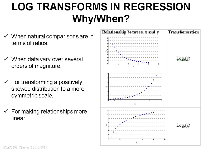
STAT6202 Chapter 2 2012/2013 24 LOG TRANSFORMS IN REGRESSION Why/When? When natural comparisons are in terms of ratios. When data vary over several orders of magniture. For transforming a positively skewed distribution to a more symmetric scale. For making relationships more linear:

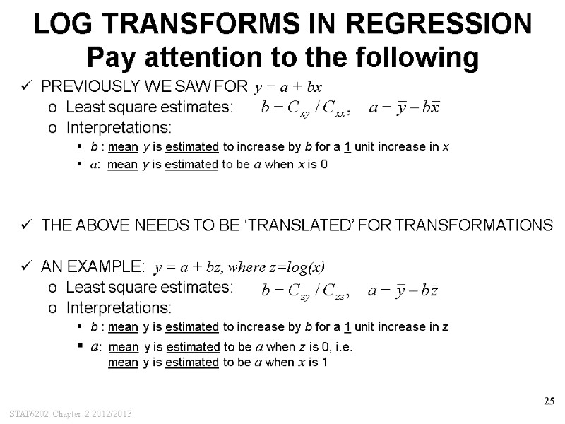
STAT6202 Chapter 2 2012/2013 25 PREVIOUSLY WE SAW FOR y = a + bx Least square estimates: Interpretations: b : mean y is estimated to increase by b for a 1 unit increase in x a: mean y is estimated to be a when x is 0 THE ABOVE NEEDS TO BE ‘TRANSLATED’ FOR TRANSFORMATIONS AN EXAMPLE: y = a + bz, where z=log(x) Least square estimates: Interpretations: b : mean y is estimated to increase by b for a 1 unit increase in z a: mean y is estimated to be a when z is 0, i.e. mean y is estimated to be a when x is 1 LOG TRANSFORMS IN REGRESSION Pay attention to the following

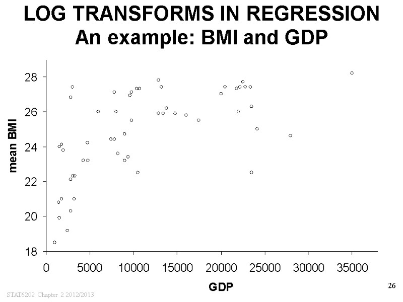
STAT6202 Chapter 2 2012/2013 26 LOG TRANSFORMS IN REGRESSION An example: BMI and GDP

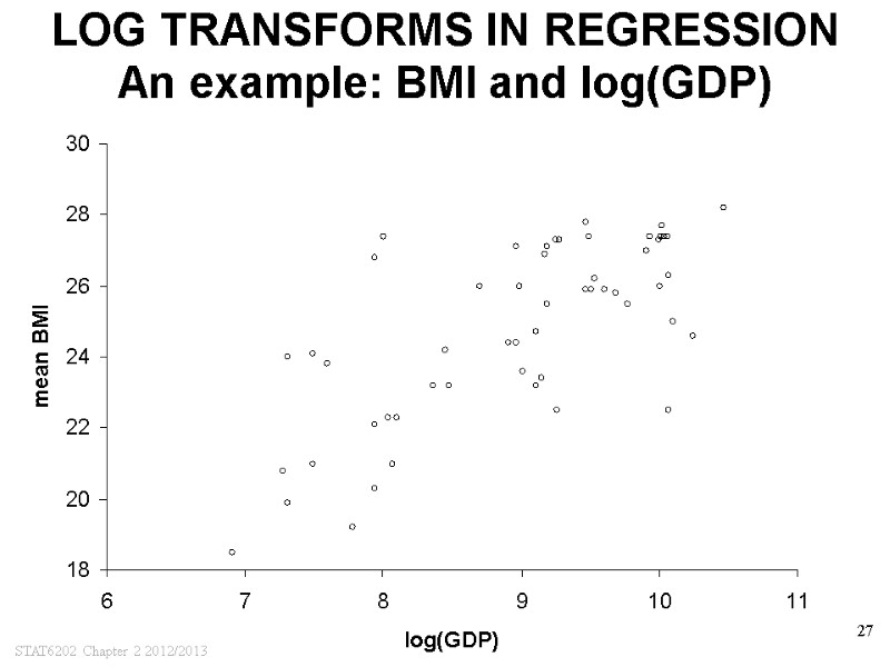
STAT6202 Chapter 2 2012/2013 27 LOG TRANSFORMS IN REGRESSION An example: BMI and log(GDP)

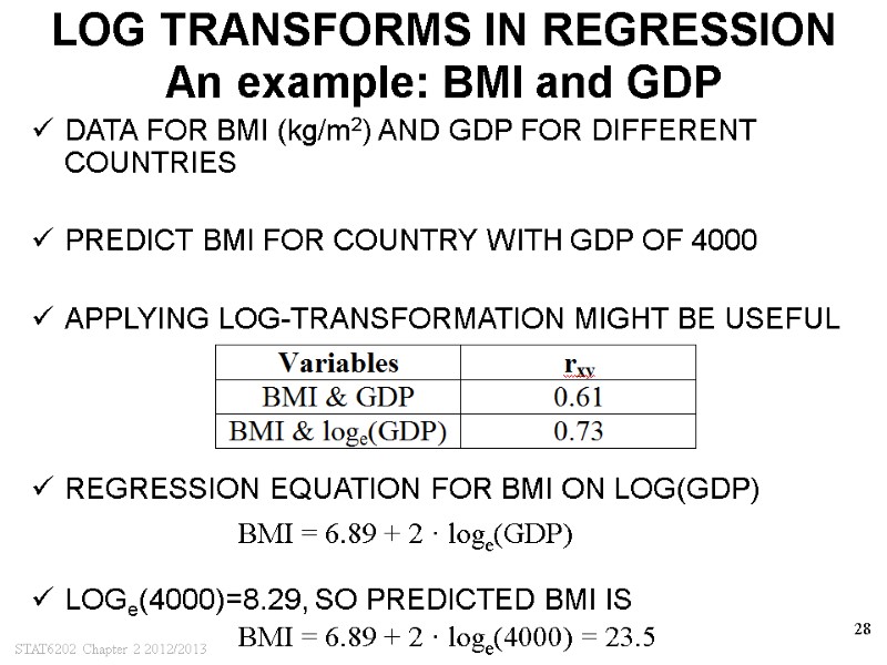
STAT6202 Chapter 2 2012/2013 28 LOG TRANSFORMS IN REGRESSION An example: BMI and GDP DATA FOR BMI (kg/m2) AND GDP FOR DIFFERENT COUNTRIES PREDICT BMI FOR COUNTRY WITH GDP OF 4000 APPLYING LOG-TRANSFORMATION MIGHT BE USEFUL REGRESSION EQUATION FOR BMI ON LOG(GDP) LOGe(4000)=8.29, SO PREDICTED BMI IS BMI = 6.89 + 2 · loge(4000) = 23.5 BMI = 6.89 + 2 · loge(GDP)

STAT6202 Chapter 2 2012/2013 29 CHAPTER 2 Describing bivariate data NOTATION SCATTER PLOT SIMPLE LINEAR REGRESSION What is it? Least squares estimation Watch out! Log transformation and regression A practical approach SAMPLE CORRELATION COEFFICIENT RANK CORRELATION COEFICIENT

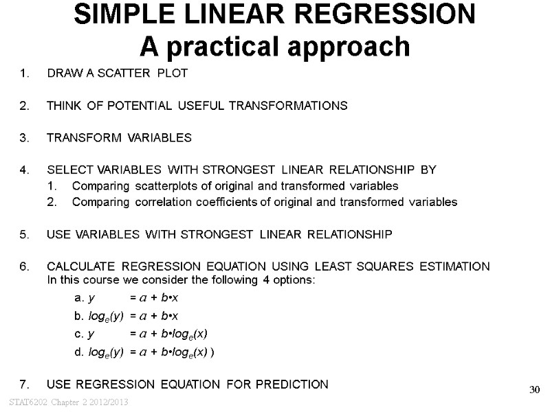
STAT6202 Chapter 2 2012/2013 30 SIMPLE LINEAR REGRESSION A practical approach DRAW A SCATTER PLOT THINK OF POTENTIAL USEFUL TRANSFORMATIONS TRANSFORM VARIABLES SELECT VARIABLES WITH STRONGEST LINEAR RELATIONSHIP BY Comparing scatterplots of original and transformed variables Comparing correlation coefficients of original and transformed variables USE VARIABLES WITH STRONGEST LINEAR RELATIONSHIP CALCULATE REGRESSION EQUATION USING LEAST SQUARES ESTIMATION In this course we consider the following 4 options: a. y = a + b•x b. loge(y) = a + b•x c. y = a + b•loge(x) d. loge(y) = a + b•loge(x) ) USE REGRESSION EQUATION FOR PREDICTION

STAT6202 Chapter 2 2012/2013 31 CHAPTER 2 Describing bivariate data NOTATION SCATTER PLOT SIMPLE LINEAR REGRESSION What is it? Least squares estimation Log transformation and regression Watch out! A practical approach SAMPLE CORRELATION COEFFICIENT RANK CORRELATION COEFICIENT

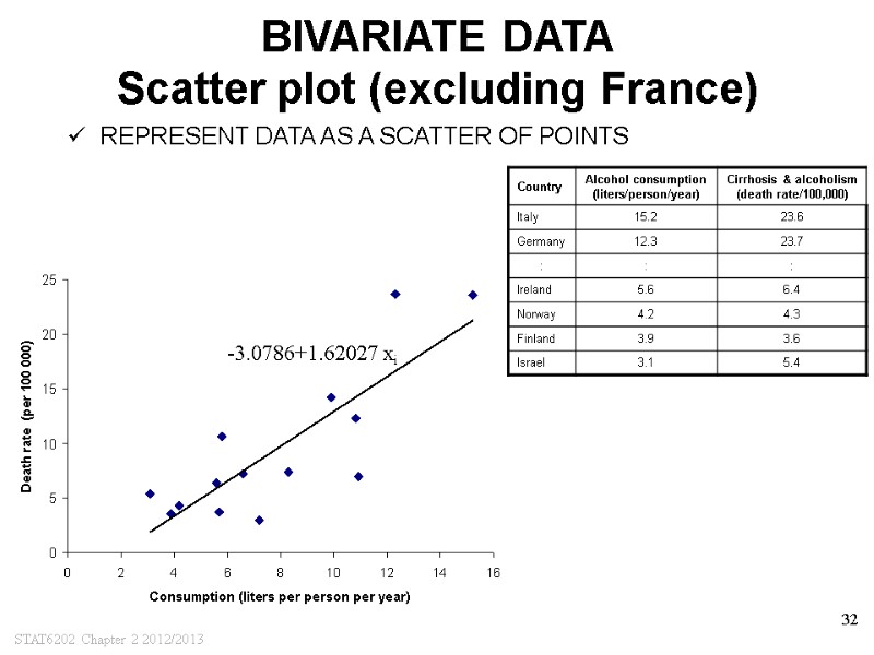
STAT6202 Chapter 2 2012/2013 32 BIVARIATE DATA Scatter plot (excluding France) REPRESENT DATA AS A SCATTER OF POINTS -3.0786+1.62027 xi

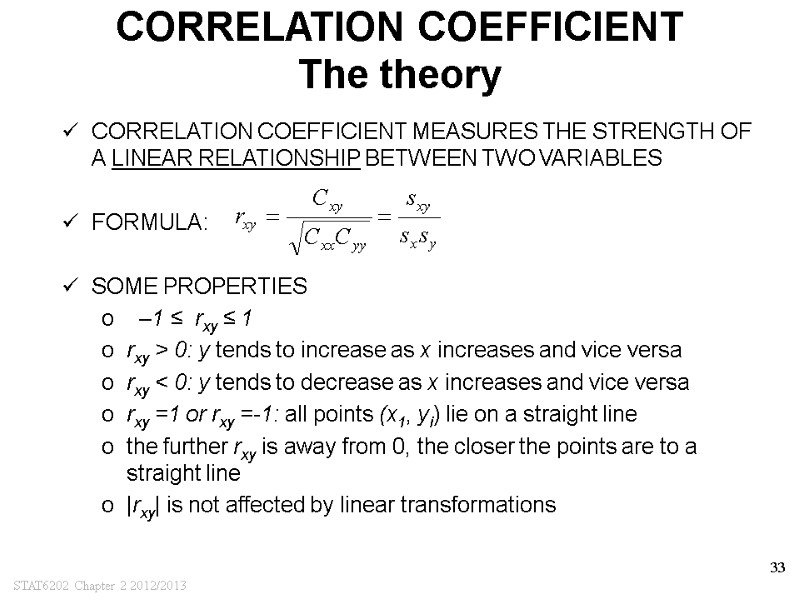
STAT6202 Chapter 2 2012/2013 33 CORRELATION COEFFICIENT The theory CORRELATION COEFFICIENT MEASURES THE STRENGTH OF A LINEAR RELATIONSHIP BETWEEN TWO VARIABLES FORMULA: SOME PROPERTIES –1 ≤ rxy ≤ 1 rxy > 0: y tends to increase as x increases and vice versa rxy < 0: y tends to decrease as x increases and vice versa rxy =1 or rxy =-1: all points (x1, yi) lie on a straight line the further rxy is away from 0, the closer the points are to a straight line |rxy| is not affected by linear transformations

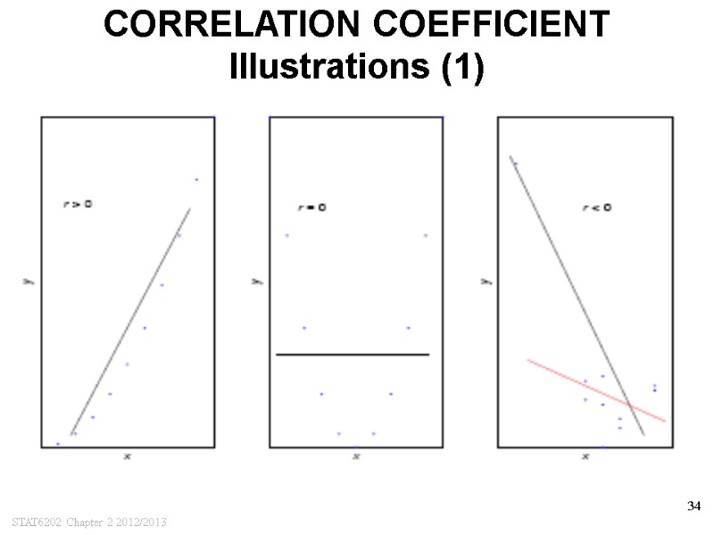
STAT6202 Chapter 2 2012/2013 34 CORRELATION COEFFICIENT Illustrations (1)

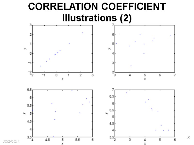
STAT6202 Chapter 2 2012/2013 35 CORRELATION COEFFICIENT Illustrations (2)

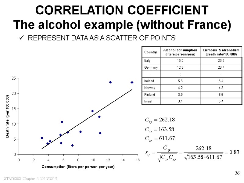
STAT6202 Chapter 2 2012/2013 36 CORRELATION COEFFICIENT The alcohol example (without France) REPRESENT DATA AS A SCATTER OF POINTS

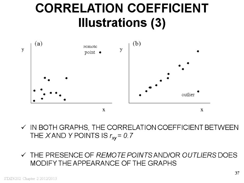
STAT6202 Chapter 2 2012/2013 37 CORRELATION COEFFICIENT Illustrations (3) IN BOTH GRAPHS, THE CORRELATION COEFFICIENT BETWEEN THE X AND Y POINTS IS rxy = 0.7 THE PRESENCE OF REMOTE POINTS AND/OR OUTLIERS DOES MODIFY THE APPEARANCE OF THE GRAPHS

STAT6202 Chapter 2 2012/2013 38 CHAPTER 2 Describing bivariate data NOTATION SCATTER PLOT SIMPLE LINEAR REGRESSION What is it? Least squares estimation Log transformation and regression Watch out! A practical approach SAMPLE CORRELATION COEFFICIENT RANK CORRELATION COEFICIENT

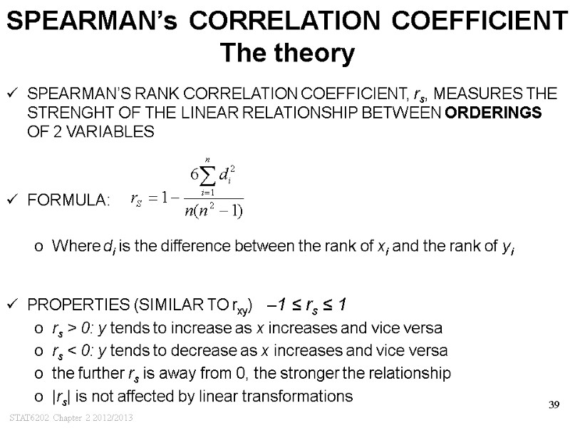
STAT6202 Chapter 2 2012/2013 39 SPEARMAN’s CORRELATION COEFFICIENT The theory SPEARMAN’S RANK CORRELATION COEFFICIENT, rs, MEASURES THE STRENGHT OF THE LINEAR RELATIONSHIP BETWEEN ORDERINGS OF 2 VARIABLES FORMULA: Where di is the difference between the rank of xi and the rank of yi PROPERTIES (SIMILAR TO rxy) –1 ≤ rs ≤ 1 rs > 0: y tends to increase as x increases and vice versa rs < 0: y tends to decrease as x increases and vice versa the further rs is away from 0, the stronger the relationship |rs| is not affected by linear transformations

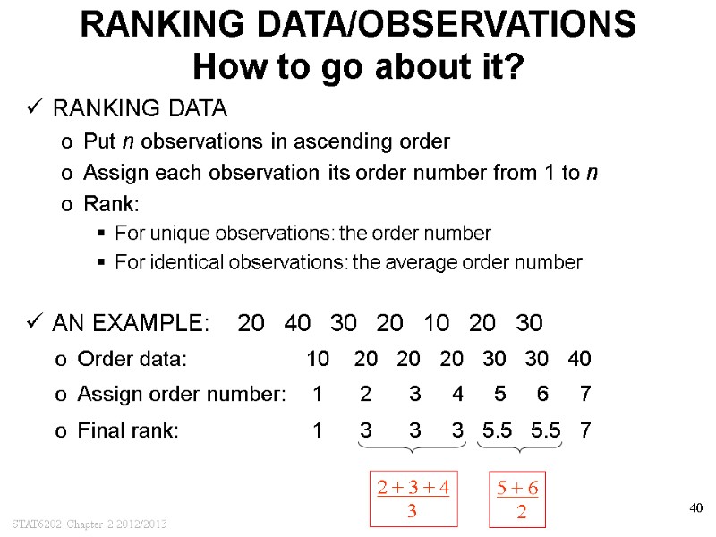
STAT6202 Chapter 2 2012/2013 40 RANKING DATA/OBSERVATIONS How to go about it? RANKING DATA Put n observations in ascending order Assign each observation its order number from 1 to n Rank: For unique observations: the order number For identical observations: the average order number AN EXAMPLE: 20 40 30 20 10 20 30 Order data: 10 20 20 20 30 30 40 Assign order number: 1 2 3 4 5 6 7 Final rank: 1 3 3 3 5.5 5.5 7 2 + 3 + 4 3 5 + 6 2

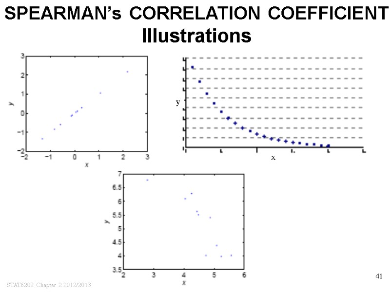
STAT6202 Chapter 2 2012/2013 41 SPEARMAN’s CORRELATION COEFFICIENT Illustrations

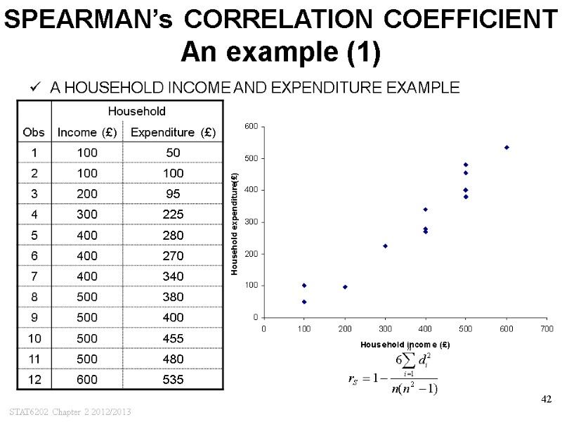
STAT6202 Chapter 2 2012/2013 42 SPEARMAN’s CORRELATION COEFFICIENT An example (1) A HOUSEHOLD INCOME AND EXPENDITURE EXAMPLE

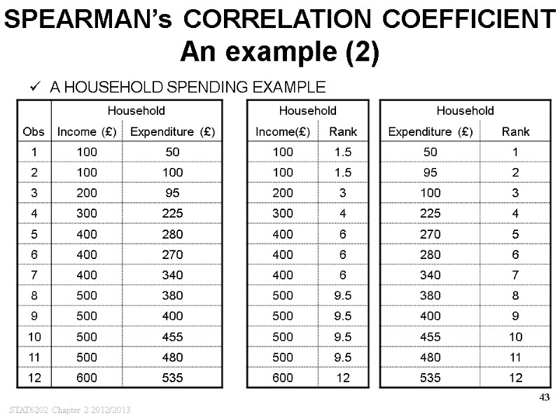
STAT6202 Chapter 2 2012/2013 43 SPEARMAN’s CORRELATION COEFFICIENT An example (2) A HOUSEHOLD SPENDING EXAMPLE

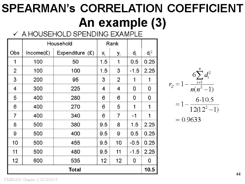
STAT6202 Chapter 2 2012/2013 44 SPEARMAN’s CORRELATION COEFFICIENT An example (3) A HOUSEHOLD SPENDING EXAMPLE