b37bfd09799e62fd10c0f55b05313801.ppt
- Количество слайдов: 55
 Stat 31, Section 1, Last Time • Independence – – • Special Case of “And” Rule Relation to Mutually Exclusive Random Variables – – – Discrete vs. Continuous Tables of Probabilities for Discrete R. V. s Areas as Probabilities for Continuous R. V. s
 Means and Variances (of random variables) Text, Sec. 4. 4 Idea: Above population summaries, extended from populations to probability distributions Connection: frequentist view Make repeated draws, from the distribution
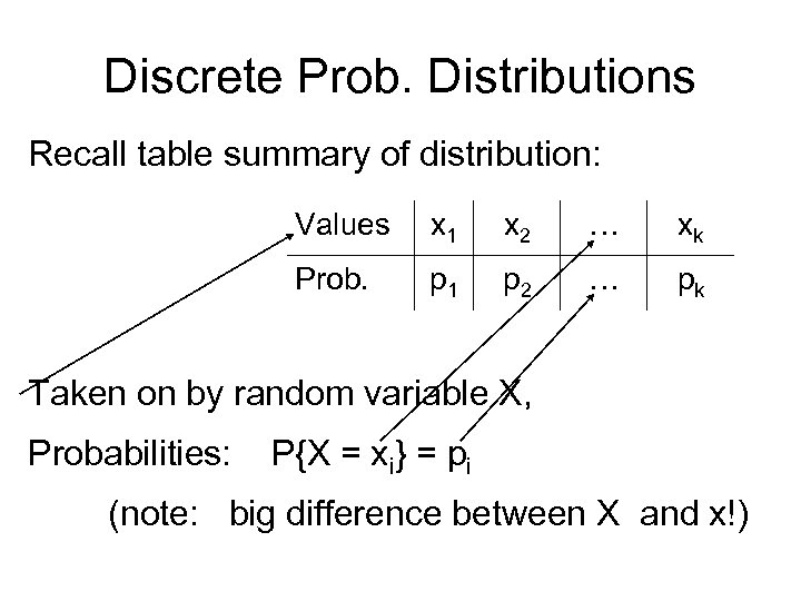 Discrete Prob. Distributions Recall table summary of distribution: Values x 1 x 2 … xk Prob. p 1 p 2 … pk Taken on by random variable X, Probabilities: P{X = xi} = pi (note: big difference between X and x!)
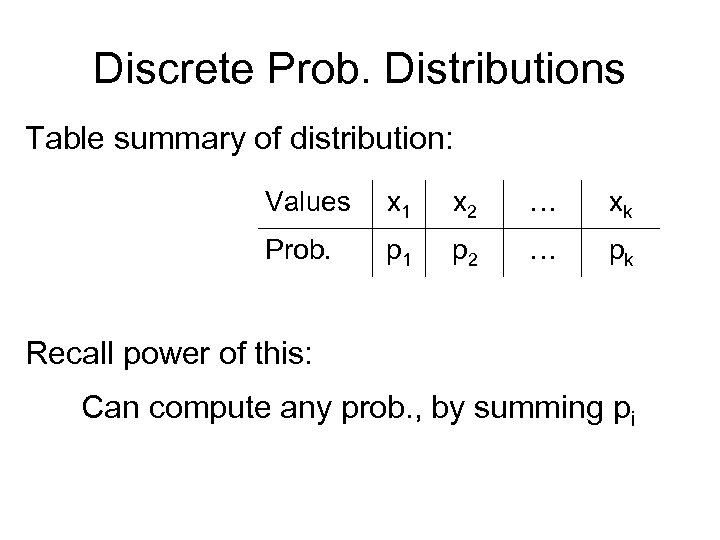 Discrete Prob. Distributions Table summary of distribution: Values x 1 x 2 … xk Prob. p 1 p 2 … pk Recall power of this: Can compute any prob. , by summing pi
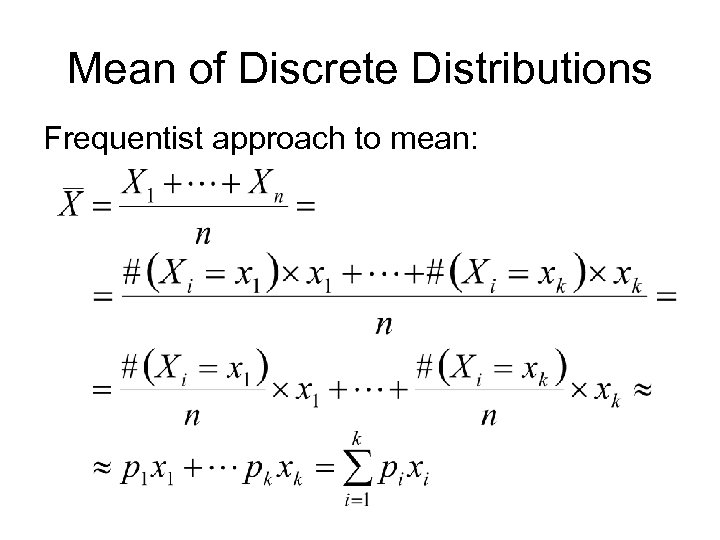 Mean of Discrete Distributions Frequentist approach to mean:
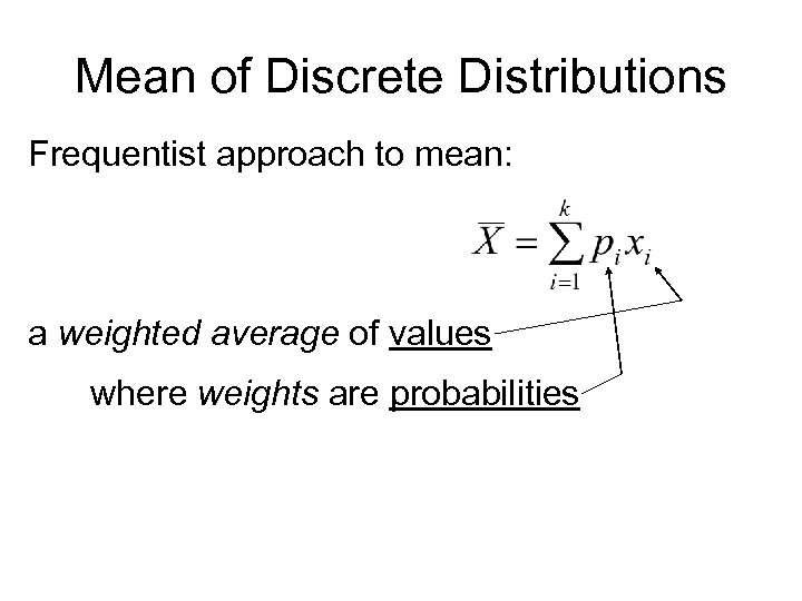 Mean of Discrete Distributions Frequentist approach to mean: a weighted average of values where weights are probabilities
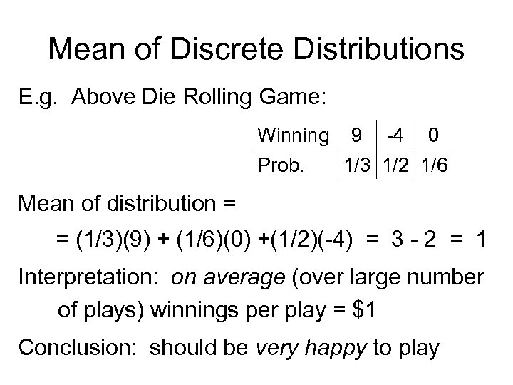 Mean of Discrete Distributions E. g. Above Die Rolling Game: Winning 9 -4 0 Prob. 1/3 1/2 1/6 Mean of distribution = = (1/3)(9) + (1/6)(0) +(1/2)(-4) = 3 - 2 = 1 Interpretation: on average (over large number of plays) winnings per play = $1 Conclusion: should be very happy to play
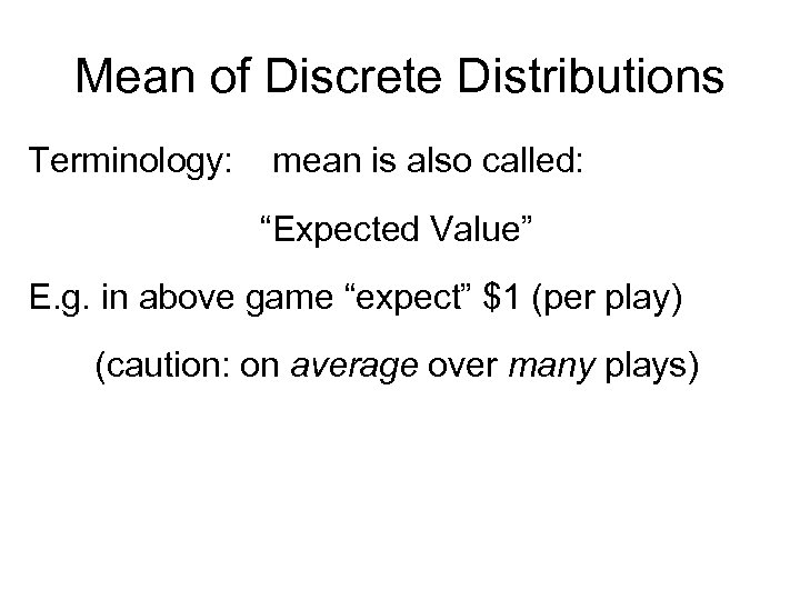 Mean of Discrete Distributions Terminology: mean is also called: “Expected Value” E. g. in above game “expect” $1 (per play) (caution: on average over many plays)
 Expected Value HW: 4. 57 4. 60 4. 61 (2. 45)
 Expected Value An application of Expected Value: Assess “fairness” of games (e. g. gambling) Major Caution: Expected Value is not what is expected on one play, but instead is average over many plays. Cannot say what happens in one or a few plays, only in long run average
 Expected Value E. g. Suppose have $5000, and need $10, 000 (e. g. you owe mafia $5000, clean out safe at work. If you give to mafia, you go to jail, so decide to try to raise additional $5000 by gambling) And can make even bets, where P{win} = 0. 48 (can really do this, e. g. bets on Red in roulette at a casino)
 Expected Value E. g. Suppose have $5000, and need $10, 000 and can make even bets, w/ P{win} = 0. 48 Pressing Practical Problem: • Should you make one large bet? • Or many small bets? • Or something in between?
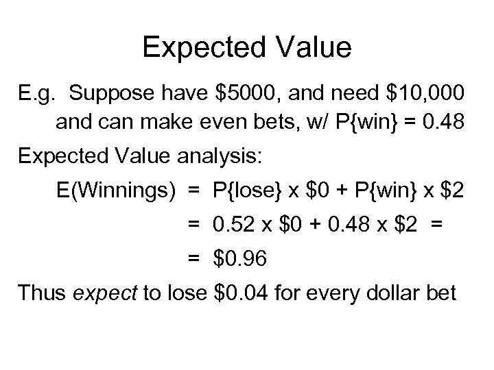 Expected Value E. g. Suppose have $5000, and need $10, 000 and can make even bets, w/ P{win} = 0. 48 Expected Value analysis: E(Winnings) = P{lose} x $0 + P{win} x $2 = 0. 52 x $0 + 0. 48 x $2 = = $0. 96 Thus expect to lose $0. 04 for every dollar bet
 Expected Value E. g. Suppose have $5000, and need $10, 000 and can make even bets, w/ P{win} = 0. 48 Expect to lose $0. 04 for every dollar bet • This is why gambling is very profitable (for the casinos, been to Las Vegas? ) • They play many times • So expected value works for them • And after many bets, you will surely lose • So should make fewer, not more bets?
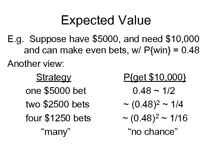 Expected Value E. g. Suppose have $5000, and need $10, 000 and can make even bets, w/ P{win} = 0. 48 Another view: Strategy P{get $10, 000} one $5000 bet 0. 48 ~ 1/2 two $2500 bets ~ (0. 48)2 ~ 1/4 four $1250 bets ~ (0. 48)2 ~ 1/16 “many” “no chance”
 Expected Value E. g. Suppose have $5000, and need $10, 000 and can make even bets, w/ P{win} = 0. 48 Surprising (? ) answer: • Best to make one big bet • Not much fun… • But best chance at winning Casino Folklore: • This really happens • Folks walk in, place one huge bet….
 Expected Value Warning about Expected Value: Excellent for some things, but not all decisions e. g. if will play many times e. g. if only play once (so don’t have long run)
 Expected Value Real life decisions against Expected Value: 1. State Lotteries – – – – State sells tickets Keeps about half of $$$ Gives rest to ~ one (randomly chosen) player So Expected Value is clearly negative Why do people play? Totally irrational? Players buy faint hope of humongous gain Could be worth joy of thinking about it
 Expected Value Real life decisions against Expected Value: 1. State Lotteries – – Want one in North Carolina? You will be asked to decide Interesting (and deep) philosophical balances: – – Only totally voluntary tax Yet tax burden borne mostly by poor Is that fair? But we lose revenue to other states…
 Expected Value Real life decisions against Expected Value: 2. Casino Gambling – – – Always lose in long run (expected value…) Yet people do it. Are they nuts? Depends on how many times they play If really enjoy being ahead sometimes Then could be worth price paid for the thrill Serious societal challenge: (some are totally consumed by thrill)
 Expected Value Real life decisions against Expected Value: 3. Insurance – – – – – Everyone pays about 2 x Expected Loss Insurance Company keeps the rest! So very profitable. But e. g. car insurance is required by law! Sensible, since if lose, can lose very big Yet purchase is totally against Expected Value OK, since you only play once (not many times) Insurance Co’s play many times (Expected Value works for them) So they are an evening out mechanism
 And now for something completely different Interesting Suggestion / Request By Katie Baer Well supported with Data / Analysis!
 SIMPLE MATH: • Date of the 2005 NCAA Men’s Basketball Tournament Final: Monday, April 4 th, 2005 • Date of the Stat 31 Midterm #2: Tuesday, April 5 th, 2005
 WHY SHOULD STEVE RESCHEDULE THE EXAM? STATISTICAL EVIDENCE:
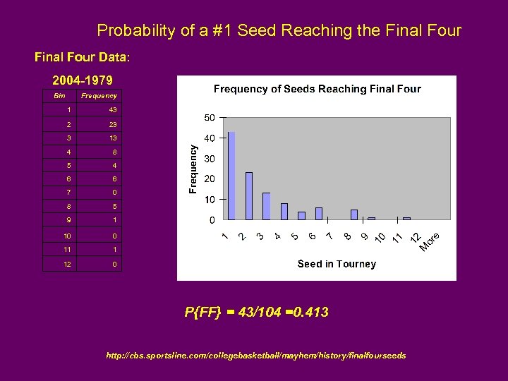 Probability of a #1 Seed Reaching the Final Four Data: 2004 -1979 Bin Frequency 1 43 2 23 3 13 4 8 5 4 6 6 7 0 8 5 9 1 10 0 11 1 12 0 P{FF} = 43/104 =0. 413 http: //cbs. sportsline. com/collegebasketball/mayhem/history/finalfourseeds
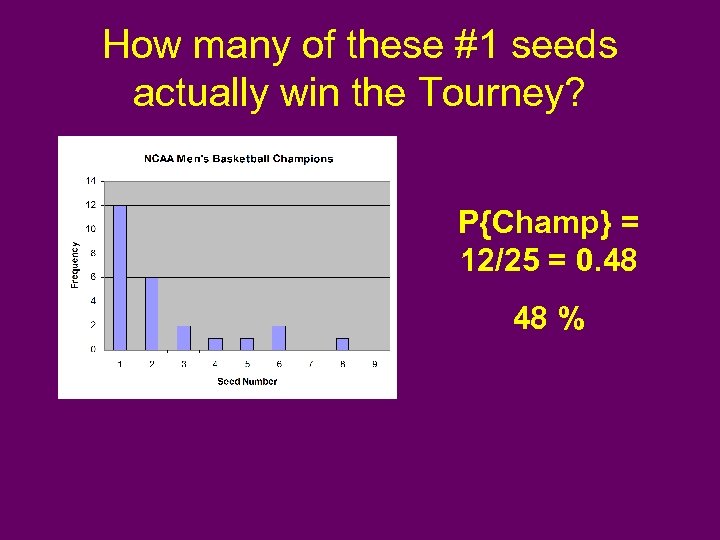 How many of these #1 seeds actually win the Tourney? P{Champ} = 12/25 = 0. 48 48 %
 However, this assumes that North Carolina has an equal probability of winning the Tourney as the other predicted #1 Seeds (Illinois, Wake Forest, and Boston College) NBC Sports, msnbc. com
 So we all know that… • Illinois is undefeated • Illinois beat Wake Forest 91 -78 and is ranked #1 in the Big 10 • Wake Forest beat North Carolina 95 -82 • North Carolina is ranked #1 in the ACC and is 4 -2 versus ranked teams • Boston College has lost only one game and is #1 in the Big Least, I mean East
 How do we determine which team is better? • RPI is derived from three component factors: Div. I winning percentage (25)%, schedule strength (50)%; and opponent's schedule strength (25)%. • How do the #1 Seeds’ RPI’s compare to the rest of the Top 25?
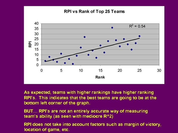 As expected, teams with higher rankings have higher ranking RPI’s. This indicates that the best teams are going to be at the bottom left corner of the graph. BUT… RPI’s are not an entirely accurate way of measuring team’s ability (as seen with mediocre R^2) RPI does not take into account factors such as margin of victory, location of game, etc.
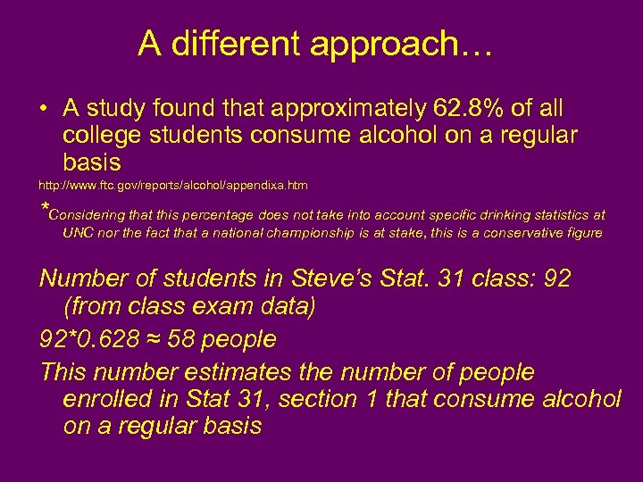 A different approach… • A study found that approximately 62. 8% of all college students consume alcohol on a regular basis http: //www. ftc. gov/reports/alcohol/appendixa. htm *Considering that this percentage does not take into account specific drinking statistics at UNC nor the fact that a national championship is at stake, this is a conservative figure Number of students in Steve’s Stat. 31 class: 92 (from class exam data) 92*0. 628 ≈ 58 people This number estimates the number of people enrolled in Stat 31, section 1 that consume alcohol on a regular basis
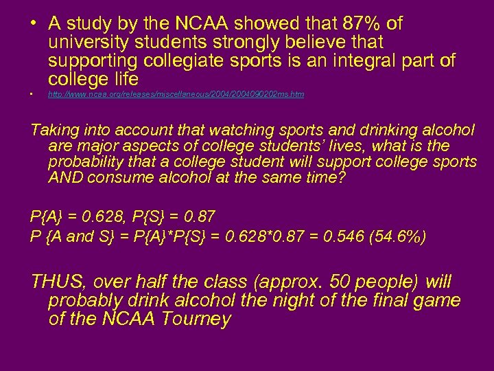 • A study by the NCAA showed that 87% of university students strongly believe that supporting collegiate sports is an integral part of college life • http: //www. ncaa. org/releases/miscellaneous/2004090202 ms. htm Taking into account that watching sports and drinking alcohol are major aspects of college students’ lives, what is the probability that a college student will support college sports AND consume alcohol at the same time? P{A} = 0. 628, P{S} = 0. 87 P {A and S} = P{A}*P{S} = 0. 628*0. 87 = 0. 546 (54. 6%) THUS, over half the class (approx. 50 people) will probably drink alcohol the night of the final game of the NCAA Tourney
 Conclusions: • Carolina has a considerable chance of reaching the Final Four and winning the NCAA tourney as a #1 seed as seen in past tournament data • They have fierce competition, as seen with in the graph of RPI vs. Rank, for the title • Over half of the class will probably consume alcohol the night of April 4 th, resulting in difficulty in studying for a midterm scheduled the next day • Note that these figures are very conservative percentages, given that students will most likely drink more when their team is in the final game and especially if it is a close, exciting match-up
 PLEASE MOVE THE TEST, STEVE! GO HEELS!!!
 And now for something completely different Now about that exam change request… • It is possible • But we all need to agree • Some choices: Thursday, April 7 • or Tuesday, April 12 Please email objections to either
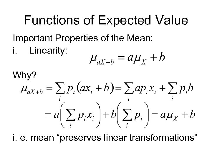 Functions of Expected Value Important Properties of the Mean: i. Linearity: Why? i. e. mean “preserves linear transformations”
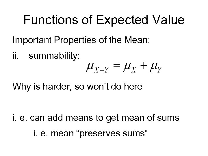 Functions of Expected Value Important Properties of the Mean: ii. summability: Why is harder, so won’t do here i. e. can add means to get mean of sums i. e. mean “preserves sums”
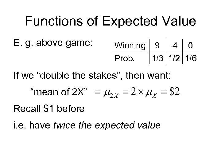 Functions of Expected Value E. g. above game: Winning 9 -4 0 Prob. 1/3 1/2 1/6 If we “double the stakes”, then want: “mean of 2 X” Recall $1 before i. e. have twice the expected value
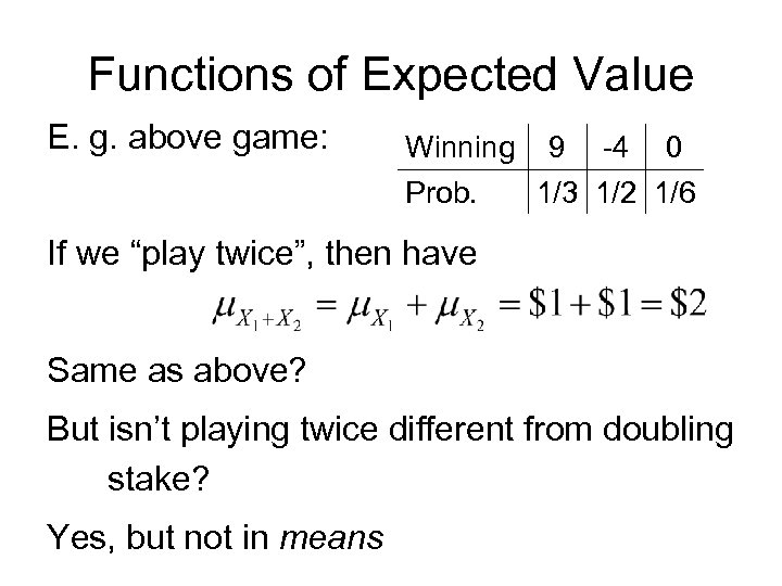 Functions of Expected Value E. g. above game: Winning 9 -4 0 Prob. 1/3 1/2 1/6 If we “play twice”, then have Same as above? But isn’t playing twice different from doubling stake? Yes, but not in means
 Functions of Expected Value HW: 4. 67 4. 68 (70)
 Indep. Of Random Variables Independence: Random Variables X & Y are independent when knowledge of value of X does not change chances of values of Y
 Indep. Of Random Variables HW: 4. 64 4. 65 (Indep. , Dep. )
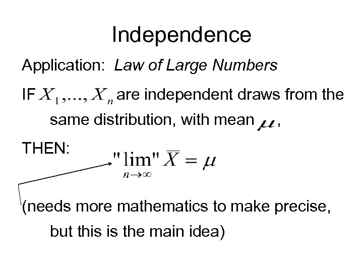 Independence Application: Law of Large Numbers IF are independent draws from the same distribution, with mean , THEN: (needs more mathematics to make precise, but this is the main idea)
 Independence Application: Law of Large Numbers Note: this is the foundation of the “frequentist view of probability” Underlying thought experiment is based on many replications, so limit works….
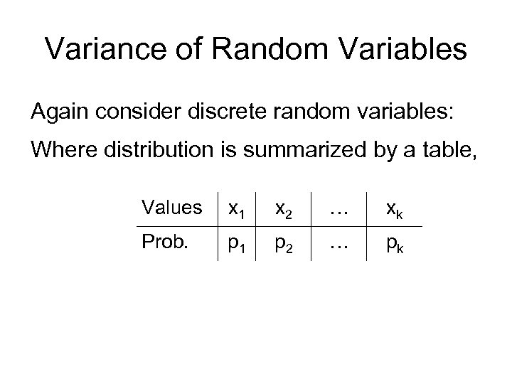 Variance of Random Variables Again consider discrete random variables: Where distribution is summarized by a table, Values x 1 x 2 … xk Prob. p 1 p 2 … pk
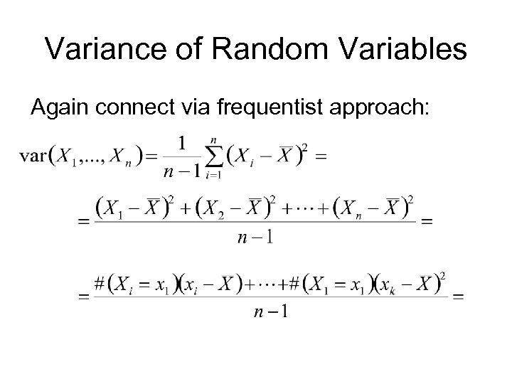 Variance of Random Variables Again connect via frequentist approach:
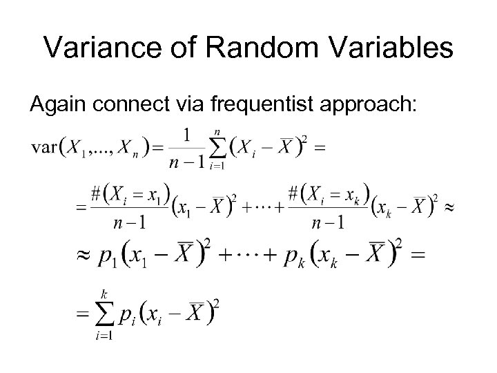 Variance of Random Variables Again connect via frequentist approach:
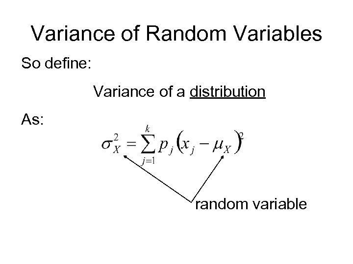 Variance of Random Variables So define: Variance of a distribution As: random variable
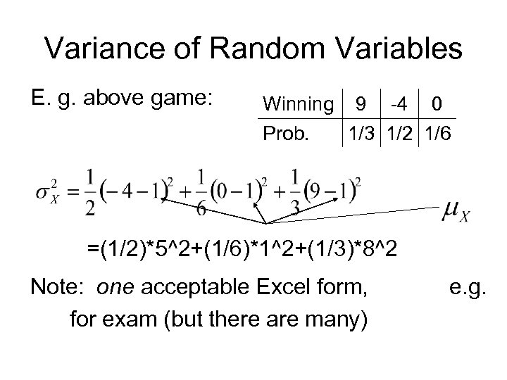 Variance of Random Variables E. g. above game: Winning 9 -4 0 Prob. 1/3 1/2 1/6 =(1/2)*5^2+(1/6)*1^2+(1/3)*8^2 Note: one acceptable Excel form, for exam (but there are many) e. g.
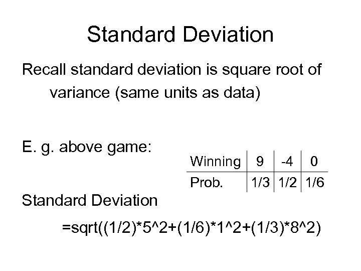 Standard Deviation Recall standard deviation is square root of variance (same units as data) E. g. above game: Winning 9 -4 0 Prob. 1/3 1/2 1/6 Standard Deviation =sqrt((1/2)*5^2+(1/6)*1^2+(1/3)*8^2)
 Variance of Random Variables HW: C 14: Find the variance and standard deviation of the distribution in 4. 60. (1. 21, 1. 10)
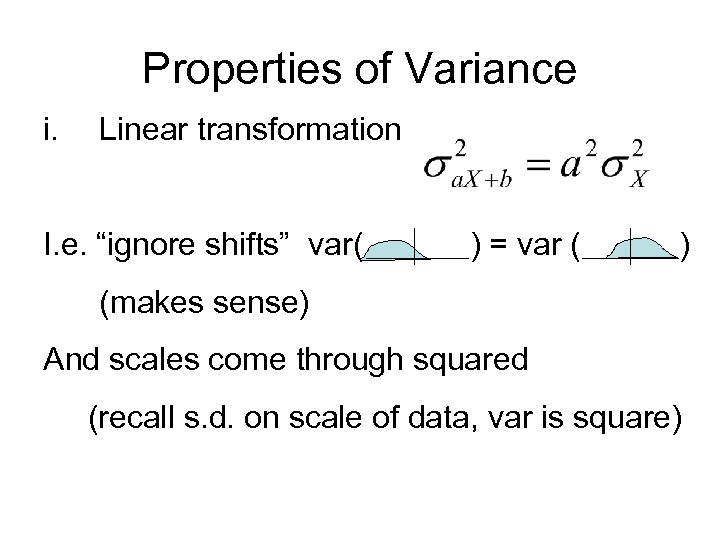 Properties of Variance i. Linear transformation I. e. “ignore shifts” var( ) = var ( ) (makes sense) And scales come through squared (recall s. d. on scale of data, var is square)
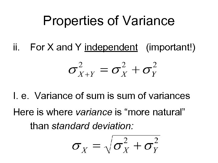 Properties of Variance ii. For X and Y independent (important!) I. e. Variance of sum is sum of variances Here is where variance is “more natural” than standard deviation:
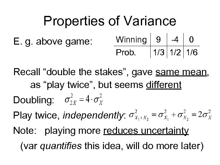 Properties of Variance E. g. above game: Winning 9 -4 0 Prob. 1/3 1/2 1/6 Recall “double the stakes”, gave same mean, as “play twice”, but seems different Doubling: Play twice, independently: Note: playing more reduces uncertainty (var quantifies this idea, will do more later)
 Variance of Random Variables HW: 4. 74 4. 75 ((a) 550, 5. 7, (b) 0, 5. 7, (c) 1022, 10. 3)


