Spring 2013 AP Microeconomics Lecture 2 Supply and

Spring 2013 AP Microeconomics Lecture 2: Supply and Demand 2/8/2018 1

Demand • Demand – The quantity consumers are willing and able to buy at each possible price during a given time period, other things constant – Amounts purchased period • at each possible price – Willing and able – Specific period – Other things constant 2

Law of Demand • Law of demand – Quantity demanded varies inversely with price, other things constant – Higher price: lower quantity demanded • Consumer Demand – Not ‘consumer wants’ – Not ‘consumer needs’ 3

Law of Demand • Substitution effect – Relative price • Price of a good relative to the prices of other goods – Lower price • Lower relative price • More willing to purchase the good 4

Law of Demand • Income effect – Money income – Real income • Measured in terms of what it can buy • Purchasing power – Lower price • Greater real income • Increase ability to purchase all goods 5

Demand Schedule and Demand Curve • Demand schedule – Possible prices – Quantity demanded at each price – Law of demand • Demand curve – Downward slope – Law of demand 6

Demand • Demand – Entire relationship between price and quantity demanded • Quantity demanded at a particular price – A point on the demand curve • Movement along the demand curve • Change in quantity demanded • Due to a change in price • Individual demand • Market demand 7

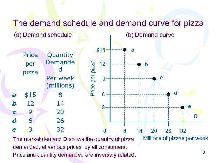The demand schedule and demand curve for pizza (b) Demand curve (a) Demand schedule a b c d e $15 12 9 6 3 Quantity Demande d Per week (millions) 8 14 20 26 32 Price per pizza a $15 12 b c 9 d 6 e 3 D 0 8 The market demand D shows the quantity of pizza demanded, at various prices, by all consumers. Price and quantity demanded are inversely related. 14 20 26 32 Millions of pizzas per week 8

Shifts of the Demand Curve 1. 2. 3. 4. Money income of consumers Prices of other goods Consumer expectations The number or composition of consumers in the market 5. Consumer tastes 9

Changes in Consumer Income • Increase in consumer income – Willing and able to buy more at each price – Increase in demand – Demand curve shifts rightward • Normal good – Demand increases as income increases • Inferior good – Demand decreases as income increases 10

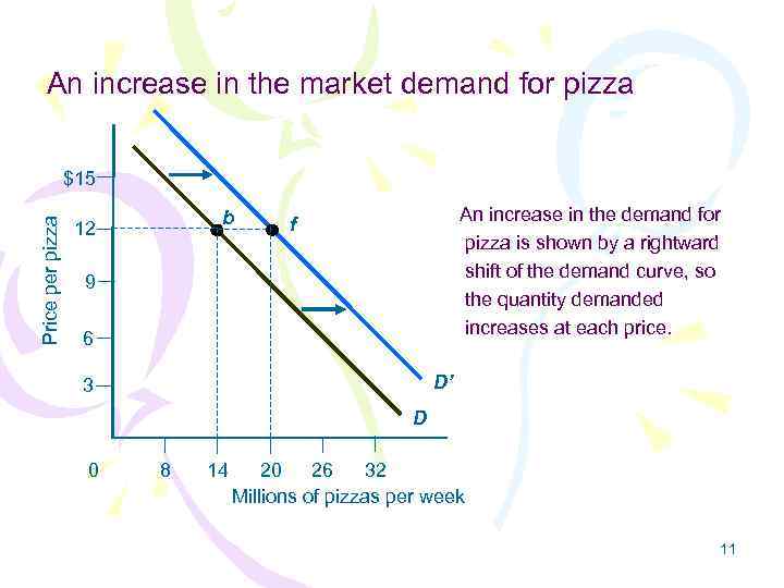An increase in the market demand for pizza Price per pizza $15 b 12 An increase in the demand for pizza is shown by a rightward shift of the demand curve, so the quantity demanded increases at each price. f 9 6 D’ 3 D 0 8 14 20 26 32 Millions of pizzas per week 11

Changes in the Prices of Other Goods • Substitutes – An increase in the price of one good • Increases the demand for the other • Rightward shift • Complements - used in combination – An increase in the price of one • Decreases the demand for the other • Leftward shift • Unrelated 12

Changes in Consumer Expectations • Income expectations – Future income increase • Increase the current demand • Price expectations – Future price increases • Increase current demand 13

Number or Composition of Consumers • Increase in number of consumers – Increases demand – Right shift • Composition of the population – Shift the demand 14

Changes in Consumer Tastes • Tastes – Likes and dislikes – Assumed given and relatively stable • Change in tastes – May shift the demand 15

Demand • Quantity demanded • Demand • Movement along the demand curve • Shift in the demand curve 16

Supply • Supply – How much producers are willing and able to offer for sale period at each possible price, other things constant – Willing and able – Specific period – Other things constant 17

Law of Supply • Law of supply – Quantity supplied is directly related to its price, other things constant – Higher price: higher quantity supplied • Higher reward, profit – More willing to increase quantity supplied; • Can afford to cover the marginal costs – Increasing opportunity cost – More able to increase quantity supplied 18

Supply Schedule and Supply Curve • Supply schedule – Possible prices – Quantity supplied at each price – Law of supply • Supply curve – Upward slope – Law of supply 19

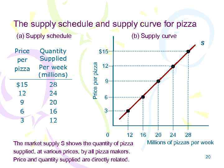The supply schedule and supply curve for pizza (b) Supply curve (a) Supply schedule S Quantity Supplied Per week (millions) $15 12 9 6 3 28 24 20 16 12 $15 Price per pizza 12 9 6 3 0 12 The market supply S shows the quantity of pizza supplied, at various prices, by all pizza makers. Price and quantity supplied are directly related. 16 20 24 28 Millions of pizzas per week 20

Supply • Supply – Entire relationship between price and quantity supplied • Quantity supplied - at a particular price – A point on the supply curve • Movement along the supply curve • Change in quantity supplied • Due to a change in price • Individual supply • Market supply 21

Shifts of the Supply Curve 1. 2. 3. 4. 5. State of technology Prices of relevant resources Prices of alternative goods Producer expectations Number of producers in the market 22

Changes in Technology • Better technology – Production costs decrease – Increase quantity supplied at each price – Increase supply – Rightward shift 23

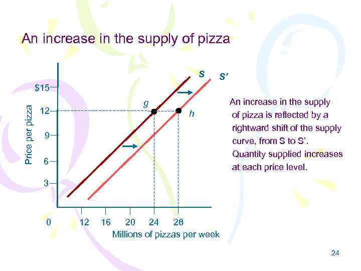An increase in the supply of pizza S S’ Price per pizza $15 g 12 h 9 6 An increase in the supply of pizza is reflected by a rightward shift of the supply curve, from S to S’. Quantity supplied increases at each price level. 3 0 12 16 20 24 28 Millions of pizzas per week 24

Prices of Relevant Resources • Relevant resources – Employed in the production • Decrease in price of relevant resources – Production costs decrease – Increase supply – Rightward shift 25

Prices of Alternative Goods • Resources – Alternative uses • Alternative goods – Use some resources employed to produce the good • Decrease in price of alternative goods – Increase supply – Rightward shift 26

Changes in Producer Expectations • Higher prices in the future – Future profits – May increase the current supply – Easily stored goods • Reduce current supply 27

Changes in the Number of Producers • Market supply – Amount supplied – At each price – By all producers • Number of producers increase – Increase supply – Rightward shift 28

Supply • Quantity supplied • Supply • Movement along the supply curve • Shift in the supply curve 29

Demand Supply Create a Market • Markets – Sort out differences between demanders and suppliers – Reduce transaction costs • Adam Smith – The “invisible hand” 30

Market Equilibrium • Surplus: excess quantity supplied – Downward pressure on price • Decrease quantity supplied • Increase quantity demanded • Shortage: excess quantity demanded – Upward pressure on price • Increase quantity supplied • Decrease quantity demanded 31

Market Equilibrium • • Quantity demanded = Quantity supplied Plans of buyers and sellers match Equilibrium point Equilibrium quantity Equilibrium price Market clears No pressure on price ‘X marks the spot’ 32

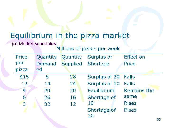Equilibrium in the pizza market (a) Market schedules Price per pizza $15 12 9 6 3 Millions of pizzas per week Quantity Demand ed Quantity Supplied 8 14 20 26 32 28 24 20 16 12 Surplus or Shortage Effect on Price Surplus of 20 Surplus of 10 Equilibrium Shortage of 10 Shortage of 20 Falls Remains the same Rises 33

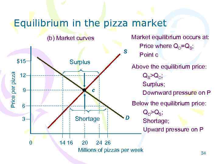Equilibrium in the pizza market (b) Market curves Price per pizza $15 Surplus 12 c 9 6 Shortage 3 0 14 16 Market equilibrium occurs at: Price where QD=QS; S Point c Above the equilibrium price: QS>QD; Surplus; Downward pressure on P Below the equilibrium price: QD>QS; D Shortage; Upward pressure on P 20 24 26 Millions of pizzas per week 34

Shifts of the Demand Curve Determinants of demand 1. 2. 3. 4. 5. Money income of consumers Price of a substitute or a complement Consumer expectations Number of consumers Consumer tastes 35

Shifts of the Demand Curve • Increase in demand – Rightward shift of D curve – Shortage; Upward pressure on P – QD decreases; QS increases – New equilibrium: Increase in P and Q • Decrease in demand – Surplus; Downward pressure on P – New equilibrium: Decrease in P and Q 36

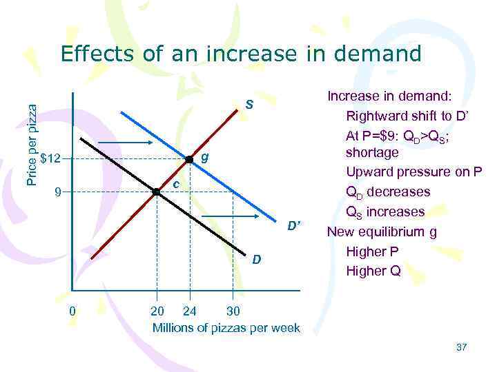Price per pizza Effects of an increase in demand S g $12 c 9 D’ D 0 Increase in demand: Rightward shift to D’ At P=$9: QD>QS; shortage Upward pressure on P QD decreases QS increases New equilibrium g Higher P Higher Q 20 24 30 Millions of pizzas per week 37

Shifts in the Supply Curve Determinants of supply 1. 2. 3. 4. 5. Technological change Price of a relevant resource Price of an alternative good Producers expectations Number of producers 38

Shifts in the Supply Curve • Increase in supply – Rightward shift of S curve – Surplus; Downward pressure on P – QD increases; QS decreases – New equilibrium: • P decreases; Q increases • Decrease in supply – New equilibrium: • P increases; Q decreases 39

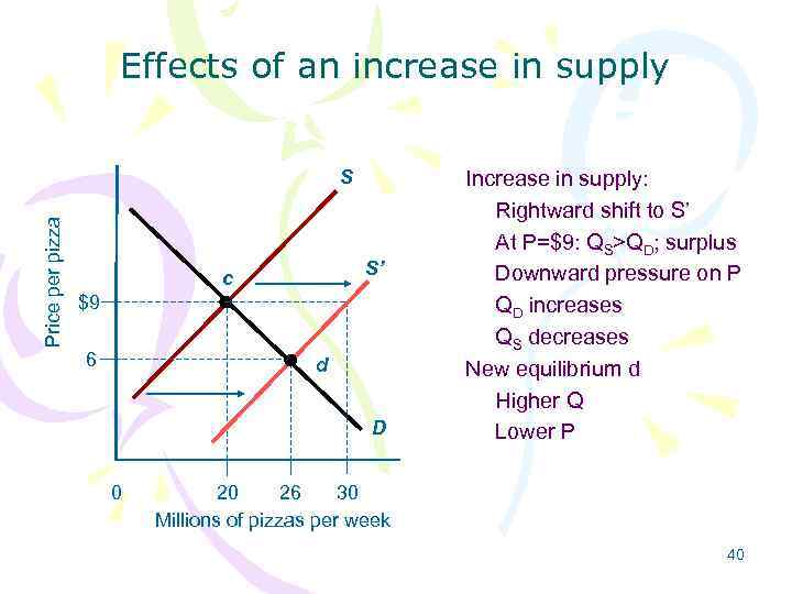Effects of an increase in supply Price per pizza S S’ c $9 6 d D 0 Increase in supply: Rightward shift to S’ At P=$9: QS>QD; surplus Downward pressure on P QD increases QS decreases New equilibrium d Higher Q Lower P 20 26 30 Millions of pizzas per week 40

Simultaneous Shifts of D and S curves • Both S and D increase: – Q increases – D shifts more: P increases – S shifts more: P decreases • Both S and D decrease: – Q decreases – D shifts more: P decreases – S shifts more: P increases 41

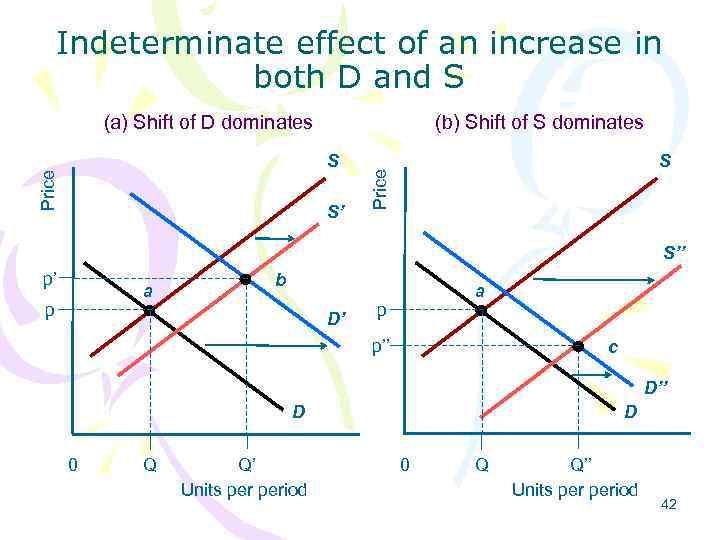Indeterminate effect of an increase in both D and S (b) Shift of S dominates (a) Shift of D dominates S’ S Price S S’’ p’ a p b D’ a p p’’ c D’’ D D 0 Q Q’ Units period 0 Q Q’’ Units period 42

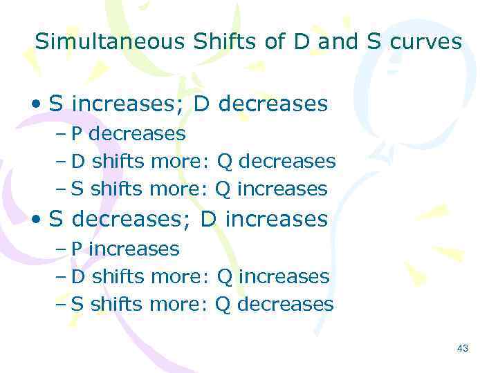Simultaneous Shifts of D and S curves • S increases; D decreases – P decreases – D shifts more: Q decreases – S shifts more: Q increases • S decreases; D increases – P increases – D shifts more: Q increases – S shifts more: Q decreases 43

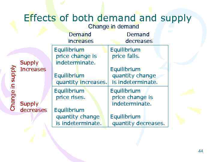Effects of both demand supply Change in demand Change in supply Demand increases Supply Increases Supply decreases Demand decreases Equilibrium price change is indeterminate. Equilibrium price falls. Equilibrium price rises. Equilibrium price change is indeterminate. Equilibrium quantity change quantity increases. is indeterminate. Equilibrium quantity change is indeterminate. Equilibrium quantity decreases. 44

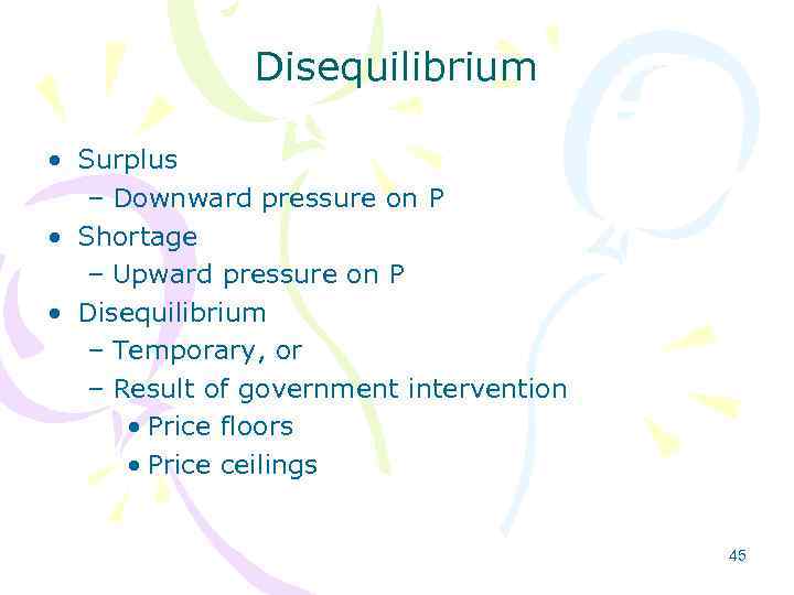Disequilibrium • Surplus – Downward pressure on P • Shortage – Upward pressure on P • Disequilibrium – Temporary, or – Result of government intervention • Price floors • Price ceilings 45

Disequilibrium • Price Floors – Set above equilibrium P – Minimum selling P – Surplus – Distort markets – Reduce economic welfare 46

Disequilibrium • Price Ceilings – Set below the equilibrium P – Maximum selling P – Shortage – Distort markets – Reduce economic welfare 47

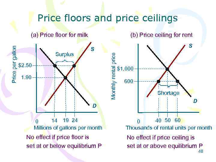Price floors and price ceilings (b) Price ceiling for rent Surplus S S Monthly rental price Price per gallon (a) Price floor for milk $2. 50 1. 90 D 14 19 24 0 Millions of gallons per month No effect if price floor is set at or below equilibrium P $1, 000 600 Shortage D 40 50 60 0 Thousands of rental units per month No effect if price ceiling is set at or above equilibrium P 48

Rent Ceilings in New York city • Rent ceilings – Housing shortage; excess demand – Drop in new construction – Decrease in quality • Increased demand in free-market sector – Higher rent – Manhattan, three-bedroom apartment • $750 if rent controlled • $12, 000 on the open market 49

Homework By doing a brief group presentation describe demand supply of any product. 50