ffbce49ca66126ec56e2b745618a24bc.ppt
- Количество слайдов: 124
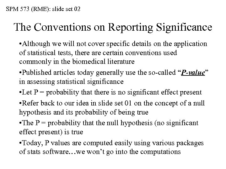 SPM 573 (RME): slide set 02 The Conventions on Reporting Significance • Although we will not cover specific details on the application of statistical tests, there are certain conventions used commonly in the biomedical literature • Published articles today generally use the so-called “P-value” in assessing statistical significance • Let P = probability that there is no significant effect present • Refer back to our idea in slide set 01 on the concept of a null hypothesis and its probability of being true • The P = probability that the null hypothesis (no significant effect present) is true • Today, P values are computed easily using various packages of stats software…we won’t go into the computations
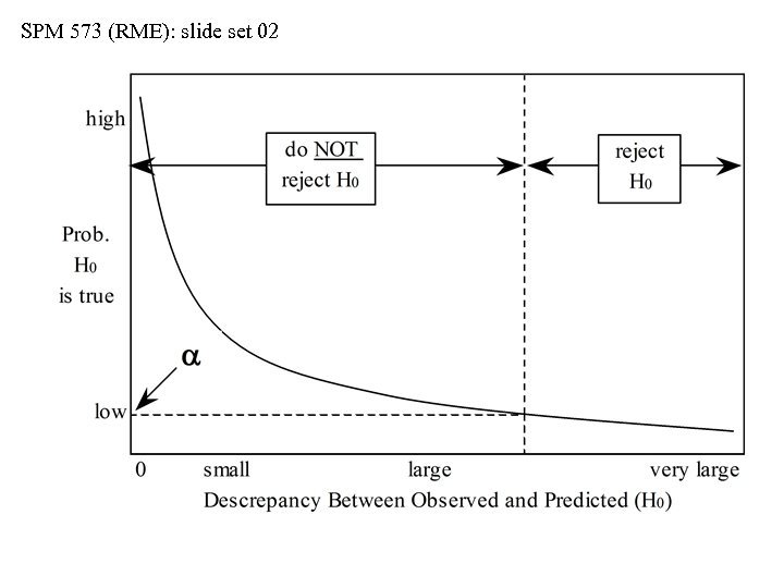 SPM 573 (RME): slide set 02
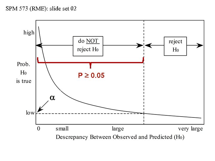 SPM 573 (RME): slide set 02 P 0. 05
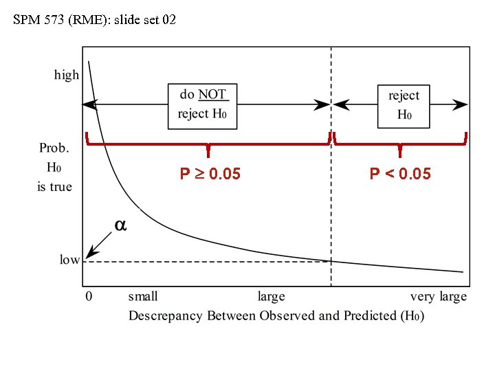 SPM 573 (RME): slide set 02 P 0. 05 P < 0. 05
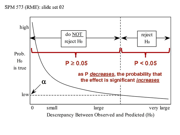 SPM 573 (RME): slide set 02 P 0. 05 P < 0. 05 as P decreases, the probability that the effect is significant increases
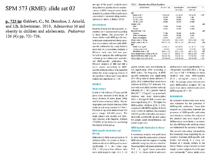 SPM 573 (RME): slide set 02 p. 723 in: Gabbert, C. , M. Donohue, J. Arnold, and J. B. Schwimmer. 2010. Adenovirus 36 and obesity in children and adolescents. Pediatrics 126 (4): pp. 721 -726.
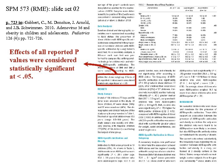 SPM 573 (RME): slide set 02 p. 723 in: Gabbert, C. , M. Donohue, J. Arnold, and J. B. Schwimmer. 2010. Adenovirus 36 and obesity in children and adolescents. Pediatrics 126 (4): pp. 721 -726. Effects of all reported P values were considered statistically significant at <. 05.
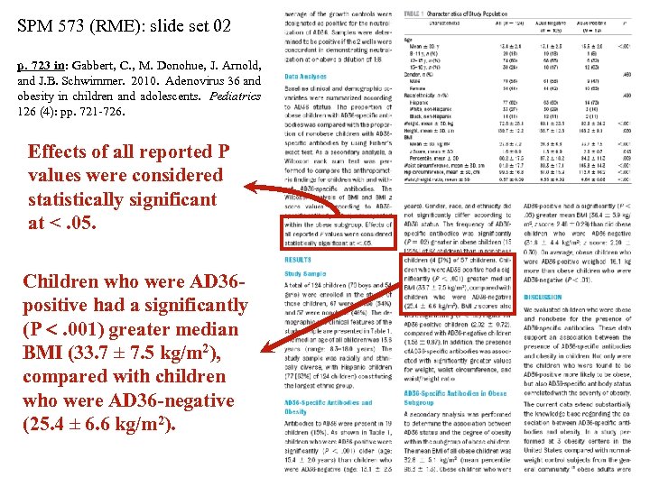 SPM 573 (RME): slide set 02 p. 723 in: Gabbert, C. , M. Donohue, J. Arnold, and J. B. Schwimmer. 2010. Adenovirus 36 and obesity in children and adolescents. Pediatrics 126 (4): pp. 721 -726. Effects of all reported P values were considered statistically significant at <. 05. Children who were AD 36 positive had a significantly (P <. 001) greater median BMI (33. 7 ± 7. 5 kg/m 2), compared with children who were AD 36 -negative (25. 4 ± 6. 6 kg/m 2).
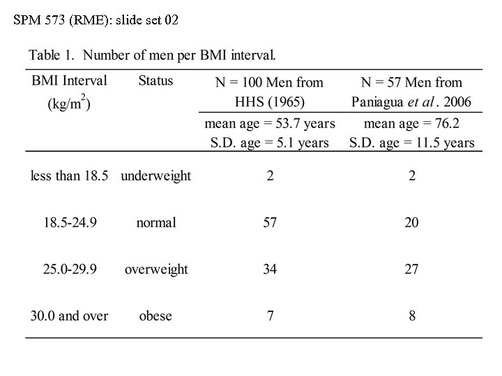
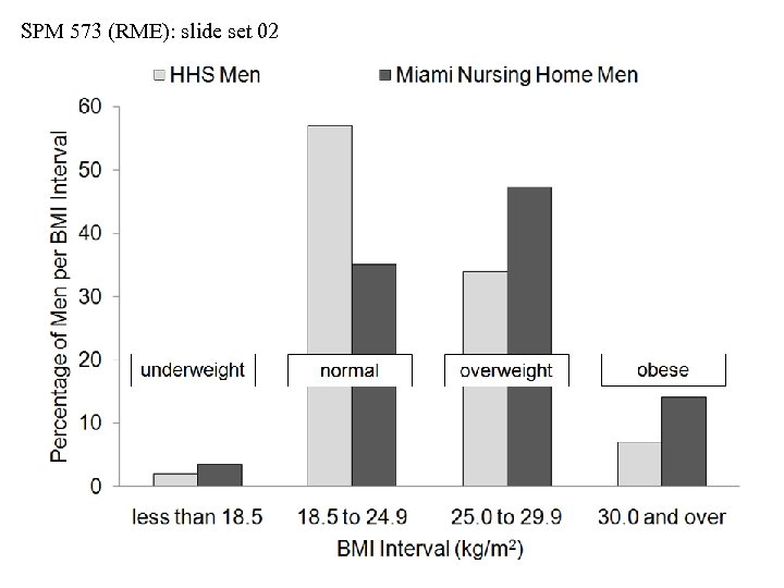
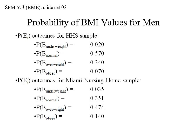
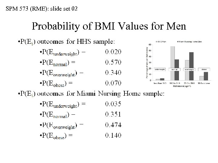
 SPM 573 (RME): slide set 02 Probability of BMI Values for Men • Some generalizations about our 65 year-old man… • 5’ 7”, 150 lb. , BMI = 23. 5 is a common value in a population of men having the HHS characteristics, but less common for men from an urban nursing home • Based on our sampling, overweight and obese men make up the majority (61%) of urban nursing home male residents • 5’ 7”, 260 lb. , BMI = 40. 7 would be a very surprising value for a man from the HHS type of population, but not as surprising for a man from an urban nursing home • Obese men are twice as common in the nursing home population as in an HHS type of population
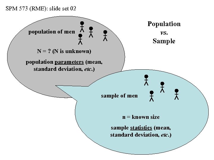 SPM 573 (RME): slide set 02 Population vs. Sample population of men N = ? (N is unknown) population parameters (mean, standard deviation, etc. ) sample of men n = known size sample statistics (mean, standard deviation, etc. )
 SPM 573 (RME): slide set 02 Meaning of Probability • Probability affects all aspects of our daily lives… • Will a hurricane strike Florida in 2014? • Will I get that internship? • Will stock market prices go up or down? • Probability applies exclusively to events in the future, but our intuition and understanding of probability rely in part on events from the past • This is a branch of mathematics that measures or estimates the likelihood that an event will have a particular outcome • Find the ratio of number of ways a specified event can occur to the total number of equally likely events that can occur
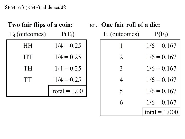
 SPM 573 (RME): slide set 02 Evaluating Probability is a Numerical Process • Ei = chance event that one specified outcome (“i”) occurs, with all possible outcomes equally likely to occur • Examples: • fair roll of a six-sided die (1, 2, 3, 4, 5, or 6 comes up) • fair flip of a two-sided coin (heads vs. tails) • Let Ei = heads (H) in a fair coin flip • P(Ei) = probability that Ei will occur • P(Ei) = P(H) = ni/N, where… • ni = number of times H comes up • N = total number of coin flips
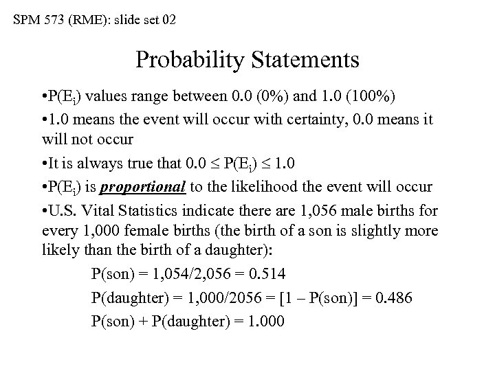 SPM 573 (RME): slide set 02 Probability Statements • P(Ei) values range between 0. 0 (0%) and 1. 0 (100%) • 1. 0 means the event will occur with certainty, 0. 0 means it will not occur • It is always true that 0. 0 P(Ei) 1. 0 • P(Ei) is proportional to the likelihood the event will occur • U. S. Vital Statistics indicate there are 1, 056 male births for every 1, 000 female births (the birth of a son is slightly more likely than the birth of a daughter): P(son) = 1, 054/2, 056 = 0. 514 P(daughter) = 1, 000/2056 = [1 – P(son)] = 0. 486 P(son) + P(daughter) = 1. 000
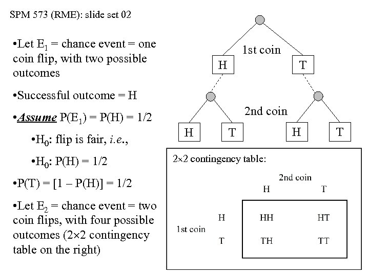 SPM 573 (RME): slide set 02 • Let E 1 = chance event = one coin flip, with two possible outcomes 1 st coin H T • Successful outcome = H • Assume P(E 1) = P(H) = 1/2 • H 0: flip is fair, i. e. , • H 0: P(H) = 1/2 • P(T) = [1 – P(H)] = 1/2 • Let E 2 = chance event = two coin flips, with four possible outcomes (2 2 contingency table on the right) 2 nd coin H T 2 2 contingency table: H T
 SPM 573 (RME): slide set 02
 SPM 573 (RME): slide set 02
 SPM 573 (RME): slide set 02
 SPM 573 (RME): slide set 02 Probability of BMI Values for Men
 SPM 573 (RME): slide set 02 Probability of BMI Values for Men
 SPM 573 (RME): slide set 02 Odds of a Florida Hurricane in 2015
 SPM 573 (RME): slide set 02
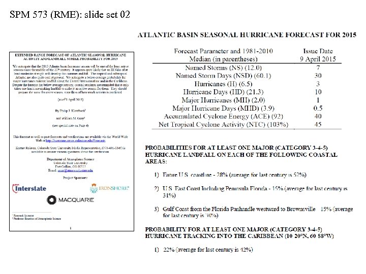
 SPM 573 (RME): slide set 02 Odds of a Florida Hurricane in 2015 • The 2015 Atlantic hurricane season is forecast now to be relatively less active with lower than average storm counts and intensities in comparison with long-term climatology records • See: Klotzbach, P. J. , and W. M. Gray. 2015. Extended range forecast of Atlantic seasonal hurricane activity and landfall strike probability for 2015 (updated 9 April 2015). • Source: http: //tropical. atmos. colostate. edu/forecasts/ • The prediction of a less active than average storm season for 2014 is based partly on two major developments… • anomalous cooling of northern Atlantic and tropical eastern Atlantic surface waters during early 2015 • high probability of El nińo weather conditions emerging in the Eastern Pacific during Summer 2015
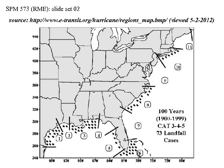 SPM 573 (RME): slide set 02 source: http: //www. e-transit. org/hurricane/regions_map. bmp/ (viewed 5 -2 -2012)
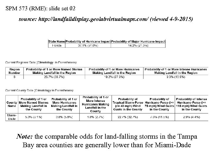 SPM 573 (RME): slide set 02 source: http: //landfalldisplay. geolabvirtualmaps. com/ (viewed 4 -9 -2015) Note: the comparable odds for land-falling storms in the Tampa Bay area counties are generally lower than for Miami-Dade
 GMS 731: slide set 02 Methods of Data Collection • Observational study: a researcher observes and measures characteristics of interest of part of a population • Experiment: a treatment is applied to part of a population, and responses are observed • Simulation: is the use of a mathematical or physical model to reproduce the conditions of a situation or process • Survey: is an investigation of one or more characteristics of a population • Census: is a measurement of an entire population • Sampling: is a measurement of part of a population
 GMS 731: slide set 02 Convenience Sampling • Sample only the population members most conveniently available (time and place), e. g. , • Patients in your assigned clinic • Students in your class • Members of your housing association • Employees in your company • Advantages: close by, very convenient and generally low cost • Disadvantages: considerable bias, homogeneous samples (people much like yourself)
 GMS 731: slide set 02 Systematic Sampling • Potential subjects are chosen and labeled at random from a large population, e. g. , a large population of men: n 1, n 2, n 3, … n 98, n 99, n 100, … nn-2, nn-1, nn • • Select a regular sampling rule, e. g. , select every fourth man: n 4, n 8, n 12, n 16, … Advantages: introduces truly random sampling Disadvatages: expensive and time-consuming, relatively heterogeneous groups • Note: this method appears commonly in the selection of subjects from lists (e. g. , phone directories, drivers licenses, etc. , which introduces the problem of those left off the lists
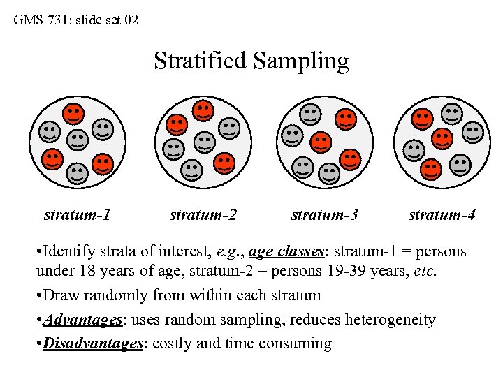 GMS 731: slide set 02 Stratified Sampling stratum-1 stratum-2 stratum-3 stratum-4 • Identify strata of interest, e. g. , age classes: stratum-1 = persons under 18 years of age, stratum-2 = persons 19 -39 years, etc. • Draw randomly from within each stratum • Advantages: uses random sampling, reduces heterogeneity • Disadvantages: costly and time consuming
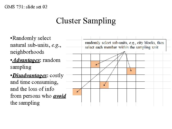 GMS 731: slide set 02 Cluster Sampling • Randomly select natural sub-units, e. g. , neighborhoods • Advantages: random sampling • Disadvantages: costly and time consuming, and the loss of info from persons who avoid the sampling
 SPM 573 (RME): slide set 02 Review of Statistical Measures • Now let’s deal with variables that are: (1) Quantitative (2) distributed in a more or less “bell-shaped” (i. e. , in a more or less Gaussian manner) • For such variables, we use measures of so-called “central tendency: ” (1) mean, (2) median, and (3) mode • We also use measures of so-called “spread” (i. e. variability): (1) range, (2) variance, (3) standard deviation, (4) standard error, and (5) coefficient of variation • Variables that are qualitative (nominal or ordinal) should NOT be viewed in any consideration of “bell-shaped” distribution
 SPM 573 (RME): slide set 02 Measure of Central Tendency • Such values locate an estimate of the so-called “middle” value among many values in the distribution • For example, line up 100 randomly selected adult American men by height (from shortest to tallest), the so-called “man in the middle” would probably be approximately 170 cm (roughly 5’ 7”) in height • The men can be ranked by height as: x 1, x 2, x 3, … x 98, x 99, x 100 • Let the height of the so-called “ith man” = xi, where i = 1, 2, … • Mean = arithmetic average value • Median = 50 th percentile value in the distribution • Mode = most frequent value in the distribution • We will compare these three values in more detail later
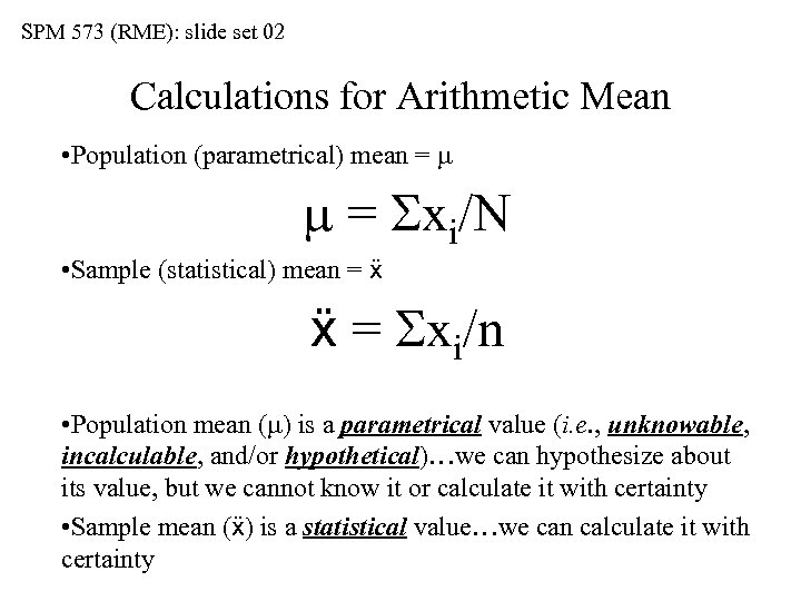 SPM 573 (RME): slide set 02 Calculations for Arithmetic Mean • Population (parametrical) mean = m m = Sxi/N • Sample (statistical) mean = ẍ ẍ = Sxi/n • Population mean (m) is a parametrical value (i. e. , unknowable, incalculable, and/or hypothetical)…we can hypothesize about its value, but we cannot know it or calculate it with certainty • Sample mean (ẍ) is a statistical value…we can calculate it with certainty
 SPM 573 (RME): slide set 02 Measures of “Spread” (Variability) • In our ranking, we use x 1, x 2, x 3, … xn-3, xn-2, xn-1, xn • In our height example, n = 100, and xn is our tallest man Range = xn – x 1 • Range is the numerical difference between tallest and shortest man in the distribution • Advantage of using range: it is a simple number, very easy to calculate • Disadvantage of using range: it uses only two values from the distribution…it ignores the other 98 values • Challenge: find a measure of spread that includes all the values in the distribution (maximizes the information)
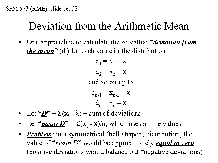 SPM 573 (RME): slide set 02 Deviation from the Arithmetic Mean • One approach is to calculate the so-called “deviation from the mean” (di) for each value in the distribution d 1 = x 1 – ẍ d 2 = x 2 – ẍ and so on up to dn-1 = xn-1 – ẍ dn = xn – ẍ • Let “D” = S(xi - ẍ) = sum of deviations • Let “mean D” = S(xi - ẍ)/n, which uses all the values • Problem: in a symmetrical (bell-shaped) distribution, the value of “mean D” would be approximately equal to zero (positive deviations would balance out “negative deviations)
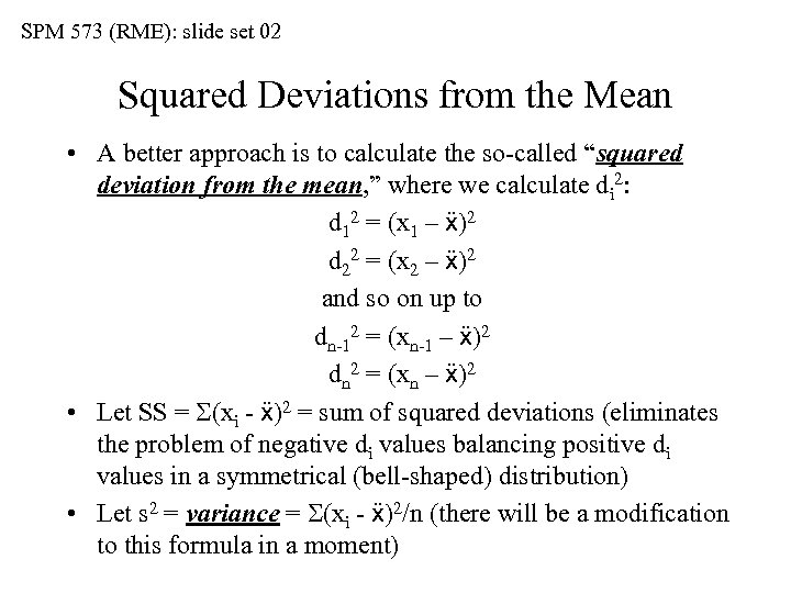 SPM 573 (RME): slide set 02 Squared Deviations from the Mean • A better approach is to calculate the so-called “squared deviation from the mean, ” where we calculate di 2: d 12 = (x 1 – ẍ)2 d 22 = (x 2 – ẍ)2 and so on up to dn-12 = (xn-1 – ẍ)2 dn 2 = (xn – ẍ)2 • Let SS = S(xi - ẍ)2 = sum of squared deviations (eliminates the problem of negative di values balancing positive di values in a symmetrical (bell-shaped) distribution) • Let s 2 = variance = S(xi - ẍ)2/n (there will be a modification to this formula in a moment)
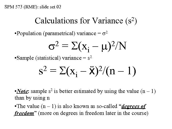 SPM 573 (RME): slide set 02 Calculations for Variance (s 2) • Population (parametrical) variance = s 2 = S(xi – m)2/N • Sample (statistical) variance = s 2 = S(xi – ẍ)2/(n – 1) • Note: sample s 2 is better estimated by using the value (n – 1) than by using n • The value (n – 1) is also known as so-called “degrees of freedom” (more on degrees in freedom later in the course)
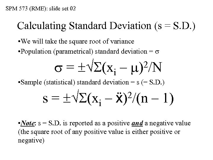 SPM 573 (RME): slide set 02 Calculating Standard Deviation (s = S. D. ) • We will take the square root of variance • Population (parametrical) standard deviation = s s = S(xi – 2/N m) • Sample (statistical) standard deviation = s (= S. D. ) s = S(xi – 2/(n ẍ) – 1) • Note: s = S. D. is reported as a positive and a negative value (the square root of any positive value is either positive or negative)
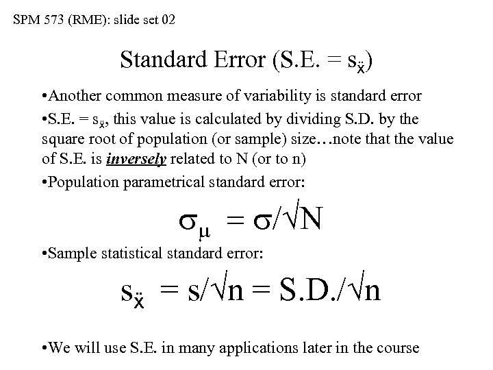 SPM 573 (RME): slide set 02 Standard Error (S. E. = sẍ) • Another common measure of variability is standard error • S. E. = sẍ, this value is calculated by dividing S. D. by the square root of population (or sample) size…note that the value of S. E. is inversely related to N (or to n) • Population parametrical standard error: sm = s/ N • Sample statistical standard error: sẍ = s/ n = S. D. / n • We will use S. E. in many applications later in the course
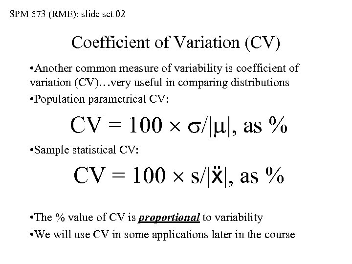 SPM 573 (RME): slide set 02 Coefficient of Variation (CV) • Another common measure of variability is coefficient of variation (CV)…very useful in comparing distributions • Population parametrical CV: CV = 100 s/|m|, as % • Sample statistical CV: CV = 100 s/|ẍ|, as % • The % value of CV is proportional to variability • We will use CV in some applications later in the course
 SPM 573 (RME): slide set 02 population of men serum cholesterol values (mg/ml)
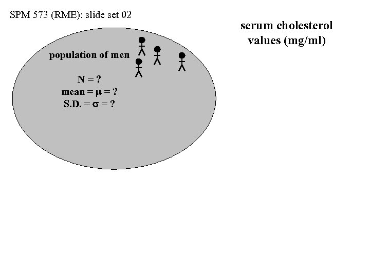 SPM 573 (RME): slide set 02 population of men N=? mean = m = ? S. D. = s = ? serum cholesterol values (mg/ml)
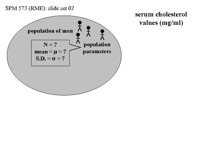 SPM 573 (RME): slide set 02 serum cholesterol values (mg/ml) population of men N=? mean = m = ? S. D. = s = ? population parameters
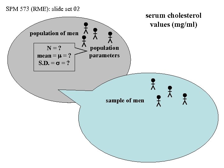 SPM 573 (RME): slide set 02 serum cholesterol values (mg/ml) population of men N=? mean = m = ? S. D. = s = ? population parameters sample of men
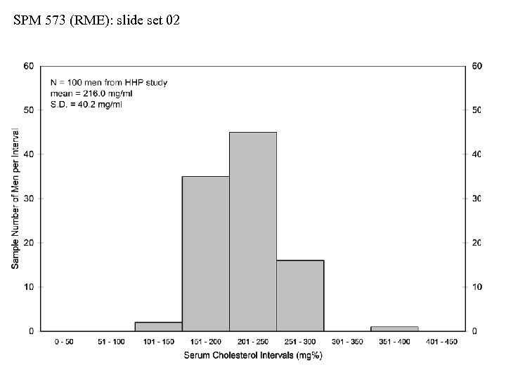
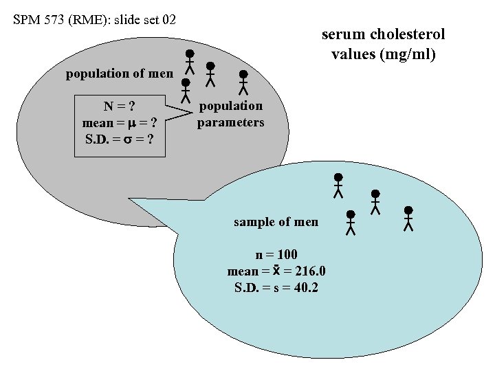 SPM 573 (RME): slide set 02 serum cholesterol values (mg/ml) population of men N=? mean = m = ? S. D. = s = ? population parameters sample of men n = 100 mean = ẍ = 216. 0 S. D. = s = 40. 2
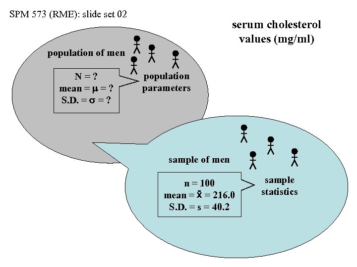 SPM 573 (RME): slide set 02 serum cholesterol values (mg/ml) population of men N=? mean = m = ? S. D. = s = ? population parameters sample of men n = 100 mean = ẍ = 216. 0 S. D. = s = 40. 2 sample statistics
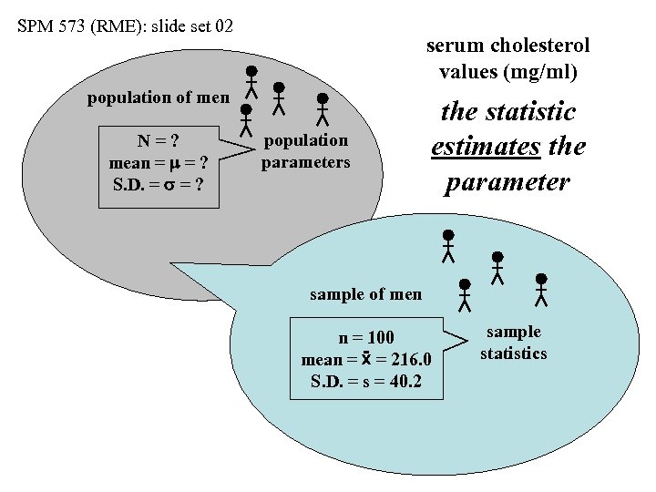 SPM 573 (RME): slide set 02 serum cholesterol values (mg/ml) population of men N=? mean = m = ? S. D. = s = ? population parameters the statistic estimates the parameter sample of men n = 100 mean = ẍ = 216. 0 S. D. = s = 40. 2 sample statistics
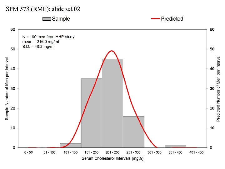
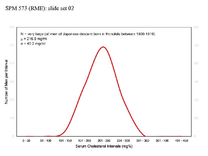
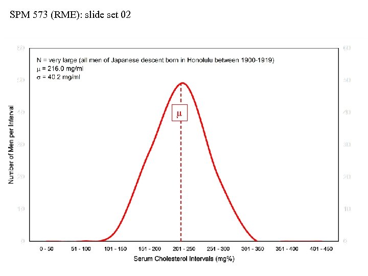
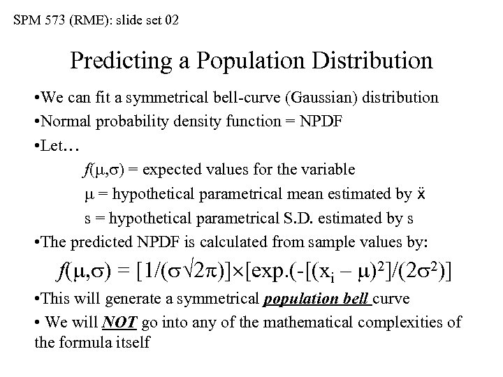 SPM 573 (RME): slide set 02 Predicting a Population Distribution • We can fit a symmetrical bell-curve (Gaussian) distribution • Normal probability density function = NPDF • Let… f(m, s) = expected values for the variable m = hypothetical parametrical mean estimated by ẍ s = hypothetical parametrical S. D. estimated by s • The predicted NPDF is calculated from sample values by: f(m, s) = [1/(s 2 )] [exp. (-[(xi – m)2]/(2 s 2)] • This will generate a symmetrical population bell curve • We will NOT go into any of the mathematical complexities of the formula itself
 SPM 573 (RME): slide set 02
 SPM 573 (RME): slide set 02
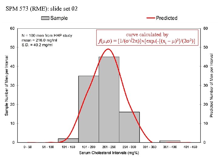 SPM 573 (RME): slide set 02 curve calculated by f(m, s) = [1/(s 2 )] [exp. (-[(xi – m)2]/(2 s 2)]
 SPM 573 (RME): slide set 02
 SPM 573 (RME): slide set 02 m
 SPM 573 (RME): slide set 02 m m 1 s
 SPM 573 (RME): slide set 02 m m 1 s m 2 s
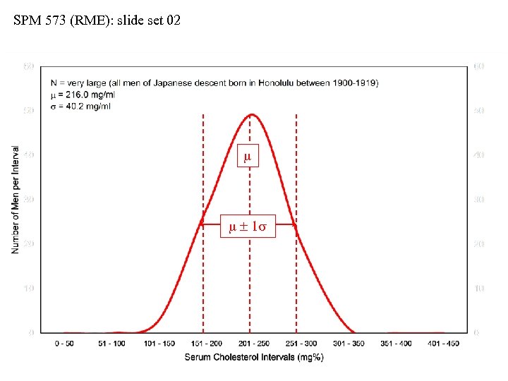
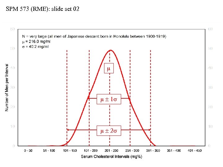
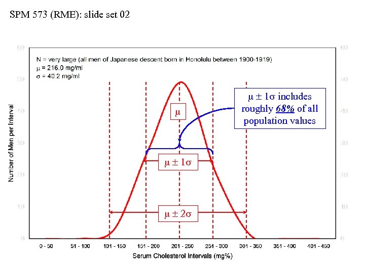 SPM 573 (RME): slide set 02 m m 1 s m 2 s m 1 s includes roughly 68% of all population values
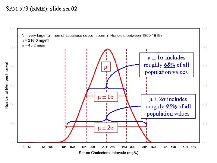 SPM 573 (RME): slide set 02 m m 1 s m 2 s m 1 s includes roughly 68% of all population values m 2 s includes roughly 95% of all population values
 SPM 573 (RME): slide set 02
 SPM 573 (RME): slide set 02
 SPM 573 (RME): slide set 02
 SPM 573 (RME): slide set 02 ẍ1 = ẍ2
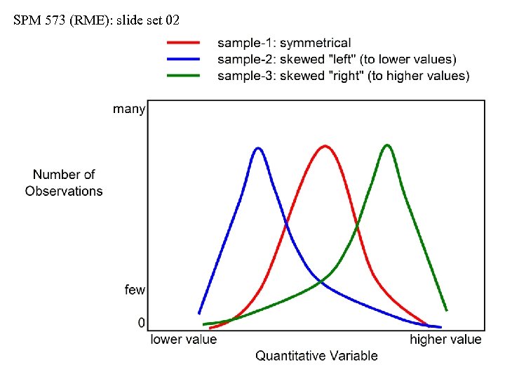
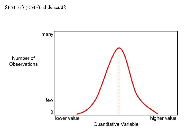
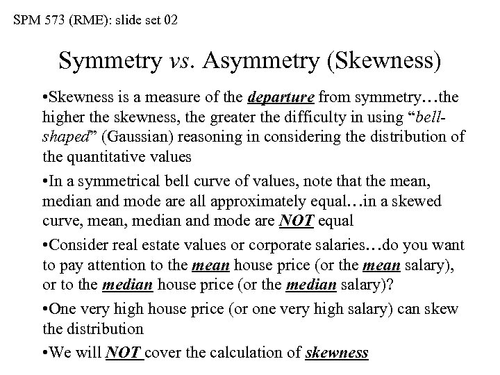 SPM 573 (RME): slide set 02 Symmetry vs. Asymmetry (Skewness) • Skewness is a measure of the departure from symmetry…the higher the skewness, the greater the difficulty in using “bellshaped” (Gaussian) reasoning in considering the distribution of the quantitative values • In a symmetrical bell curve of values, note that the mean, median and mode are all approximately equal…in a skewed curve, mean, median and mode are NOT equal • Consider real estate values or corporate salaries…do you want to pay attention to the mean house price (or the mean salary), or to the median house price (or the median salary)? • One very high house price (or one very high salary) can skew the distribution • We will NOT cover the calculation of skewness
 SPM 573 (RME): slide set 02
 SPM 573 (RME): slide set 02
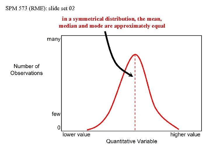 SPM 573 (RME): slide set 02 in a symmetrical distribution, the mean, median and mode are approximately equal
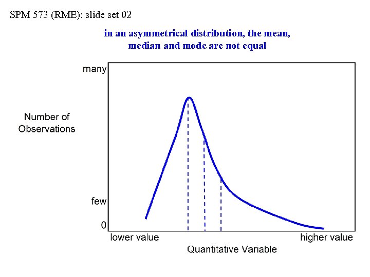 SPM 573 (RME): slide set 02 in an asymmetrical distribution, the mean, median and mode are not equal
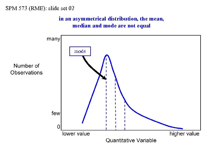 SPM 573 (RME): slide set 02 in an asymmetrical distribution, the mean, median and mode are not equal mode
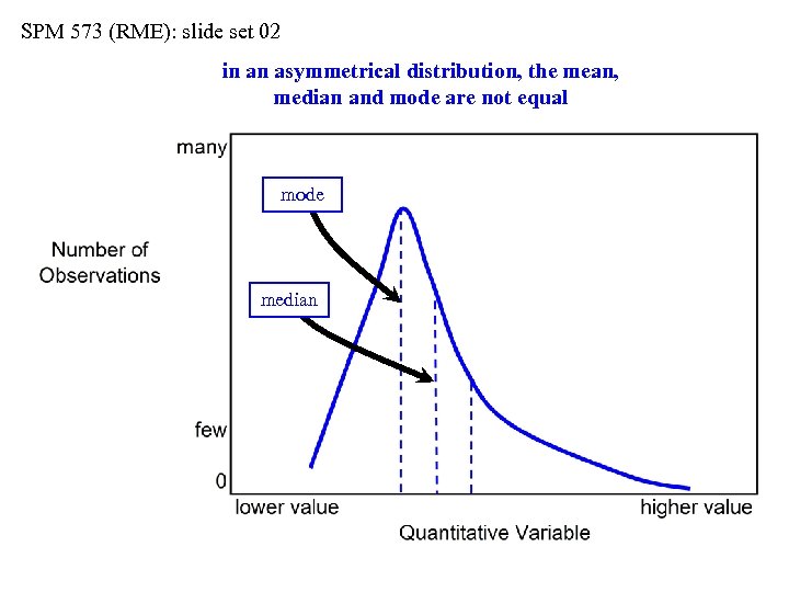 SPM 573 (RME): slide set 02 in an asymmetrical distribution, the mean, median and mode are not equal mode median
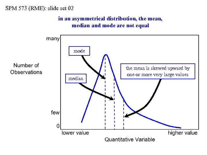 SPM 573 (RME): slide set 02 in an asymmetrical distribution, the mean, median and mode are not equal mode median the mean is skewed upward by one or more very large values
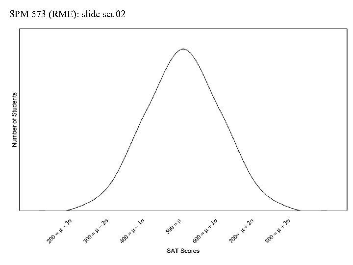
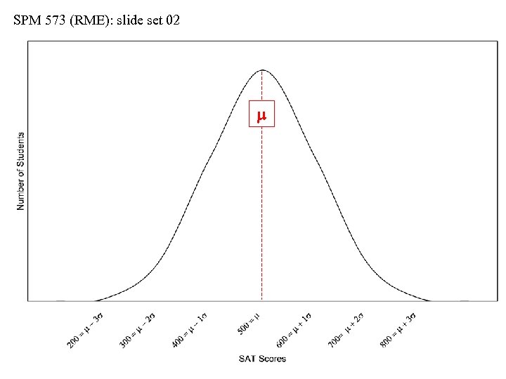
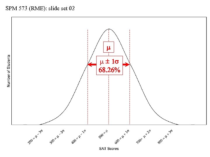
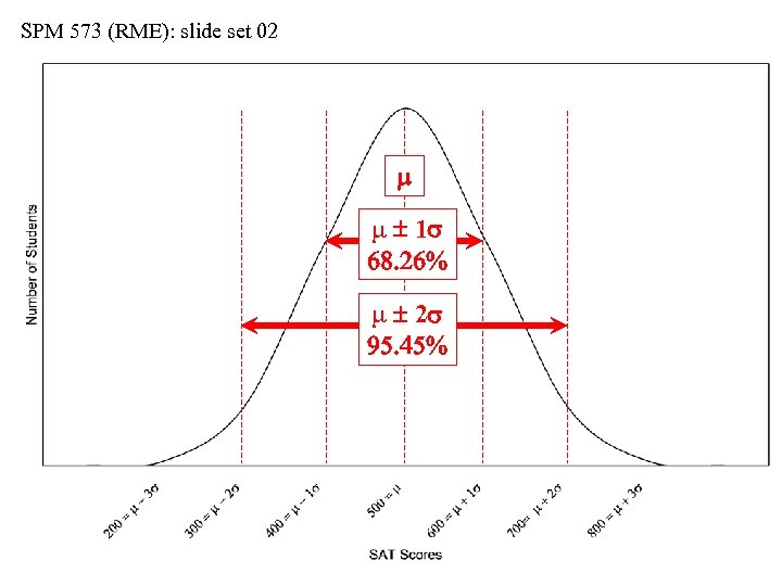
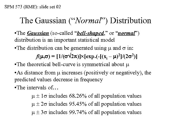 SPM 573 (RME): slide set 02 The Gaussian (“Normal”) Distribution • The Gaussian (so-called “bell-shaped, ” or “normal”) distribution is an important statistical model • The distribution can be generated using m and s in: f(m, s) = [1/(s 2 )] [exp. (-[(xi – m)2]/(2 s 2)] • The theoretical bell-curve is symmetrical about m • As distance from m increases (positively or negatively), the predicted values decrease in frequency • The intervals of… m 1 s includes 68. 26% of all population values m 2 s includes 95. 45% of all population values m 3 s includes 99. 74% of all population values
 SPM 573 (RME): slide set 02 Historical Origins • The “normal” distribution goes back nearly three centuries • It was first described as a mathematical theorem in 1733 by the Frenchman Abraham de Moivre (1667 -1754) • The French mathematician Pierre Simon de Laplace (17491827) used de Moivre’s equations to calculate probabilities • The German astronomer Carl Gauss (1777 -1855) developed de La. Place’s work into a general law of the normal probability distribution (1830’s, hence the term “Gaussian”) • During the 1890’s Francis Galton (1822 -1911) applied the general distribution to biology and medicine…Galton is sometimes referred to as the so-called “father of biostatistics” • Minor historical note: Galton was Charles Darwin’s 1 st cousin
 SPM 573 (RME): slide set 02 Example of High School SAT Scores • SAT: Scholastic Achievement Test • Developed in 1926 mainly by Carl Brigham, SAT scores are “standardized” (we will cover this process later) • The SAT has a long history of use, modification, redesign, and some controversies…we won’t go into the designs or controversies • We will consider the SAT score only as a variable that has Gaussian properties • The lowest possible SAT score (in either Verbal or Math) is 200, a score achieved by less than 1% of the test takers) • The highest possible score is 800, also a score achieved by less than 1% of the test takers
 SPM 573 (RME): slide set 02 SAT Scores in Theory • First, consider SAT scores distributed in a perfectly Gaussian manner (in practice, the national distribution tends to closely resemble the perfect Gaussian curve) • For a very large population of test takers, we will assume an average (m) score of 500 (Math or Verbal), with a standard deviation (s) of 100: • Approximately 68% of the population will lie within one s of the mean • Approximately 95% of the population will lie within two s of the mean • Approximately 99% of the population will lie within three s of the mean
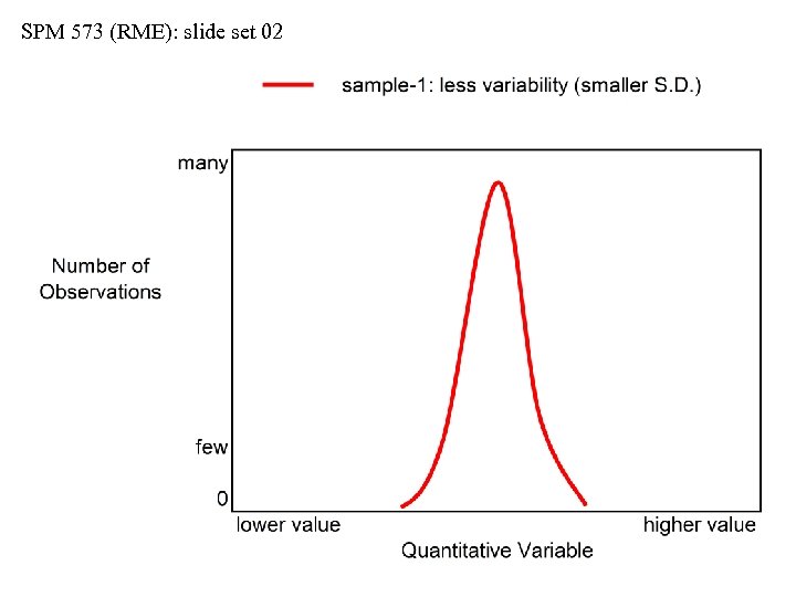
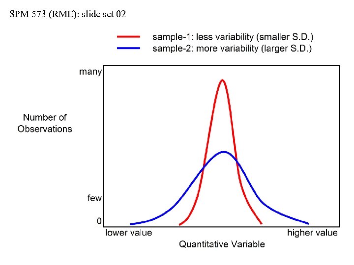
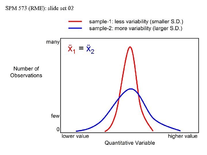
 SPM 573 (RME): slide set 02 There are Many Gaussian Curves • As we have seen, there are many Gaussian distributions for our everyday data (height, weight, SAT scores, etc. ) • Some are tall and thin (s is small), and some are short and fat (s is large) • This means that each Gaussian distribution has its own unique limits for evaluating the areas underneath the curve that will include 68%, 95% an 99% of the total values • This would make our work very complicated, but there is a solution…we can “standardize” any Gaussian distribution to a single, uniform distribution of so-called “Z-scores” • First, let’s look at some samples of SAT scores
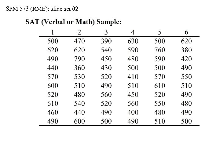
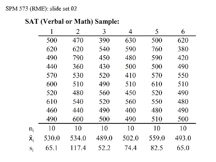
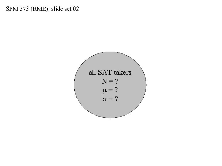
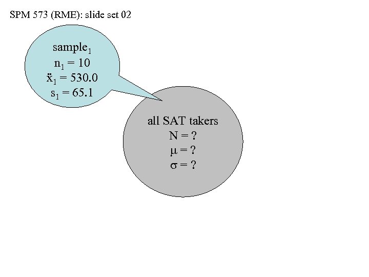
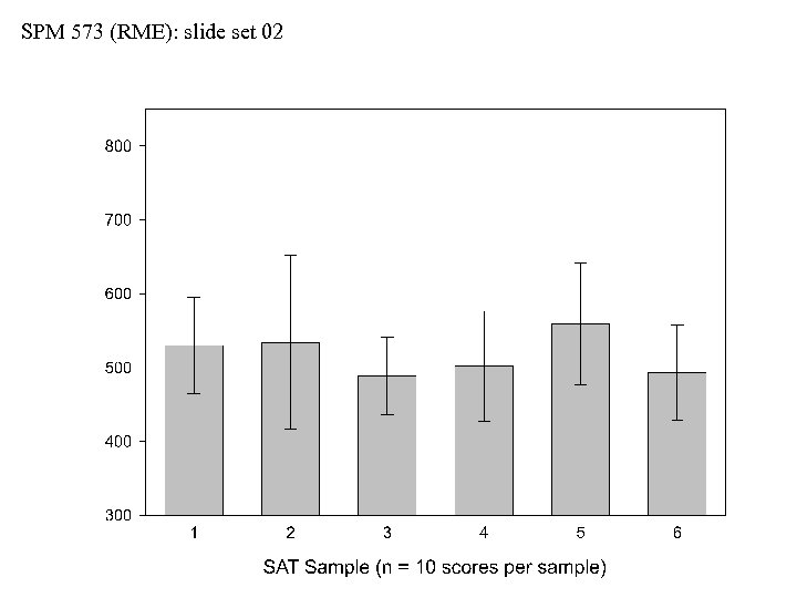
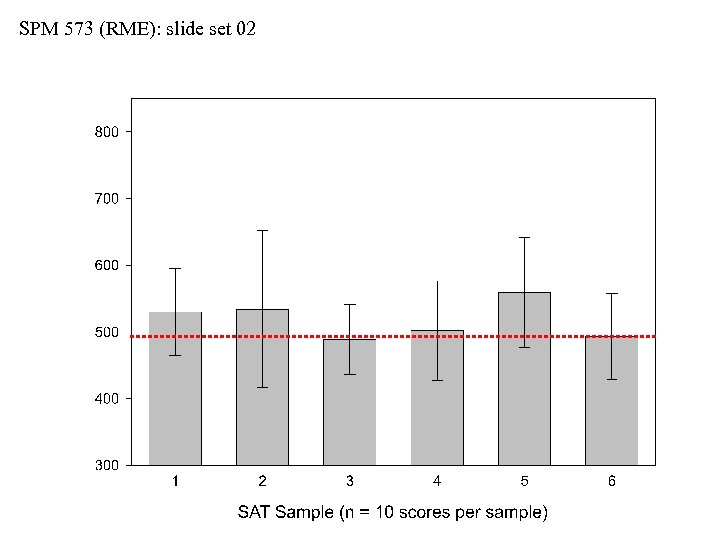
 SPM 573 (RME): slide set 02 Sampling the SAT Scores • We can select individual SAT scores (either verbal or math) at random from the national pool of data • Let’s select six samples of SAT scores, with n = 10 randomly selected scores per sample • For each sample, we’ll record the individual scores, and we’ll calculate mean and standard deviation values • Note: colleges and universities publish mean SAT’s for their incoming classes, but they rarely report measures of spread • A dirty, little secret…a university’s published SAT profile generally includes all scores for students accepted into “declared majors, ” or into “departments; ” they generally do NOT include “provisionals, ” “undeclareds, ” or “undecideds”
 SPM 573 (RME): slide set 02
 SPM 573 (RME): slide set 02
 SPM 573 (RME): slide set 02 all SAT takers N=? m=? s=?
 SPM 573 (RME): slide set 02 sample 1 n 1 = 10 ẍ1 = 530. 0 s 1 = 65. 1 all SAT takers N=? m=? s=?
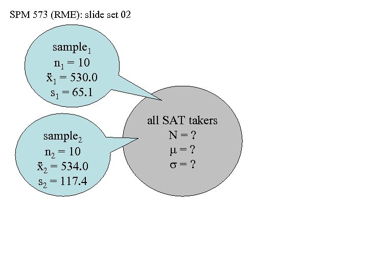 SPM 573 (RME): slide set 02 sample 1 n 1 = 10 ẍ1 = 530. 0 s 1 = 65. 1 sample 2 n 2 = 10 ẍ2 = 534. 0 s 2 = 117. 4 all SAT takers N=? m=? s=?
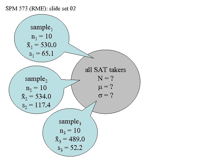 SPM 573 (RME): slide set 02 sample 1 n 1 = 10 ẍ1 = 530. 0 s 1 = 65. 1 all SAT takers N=? m=? s=? sample 2 n 2 = 10 ẍ2 = 534. 0 s 2 = 117. 4 sample 3 n 3 = 10 ẍ3 = 489. 0 s 3 = 52. 2
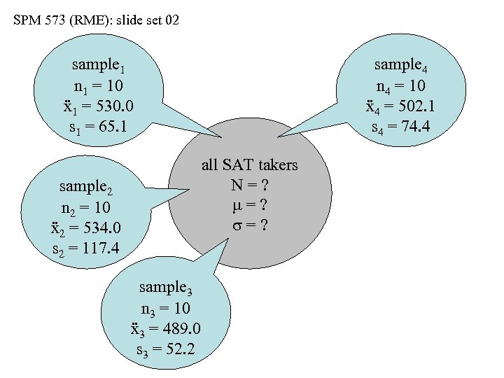 SPM 573 (RME): slide set 02 sample 1 n 1 = 10 ẍ1 = 530. 0 s 1 = 65. 1 sample 4 n 4 = 10 ẍ4 = 502. 1 s 4 = 74. 4 all SAT takers N=? m=? s=? sample 2 n 2 = 10 ẍ2 = 534. 0 s 2 = 117. 4 sample 3 n 3 = 10 ẍ3 = 489. 0 s 3 = 52. 2
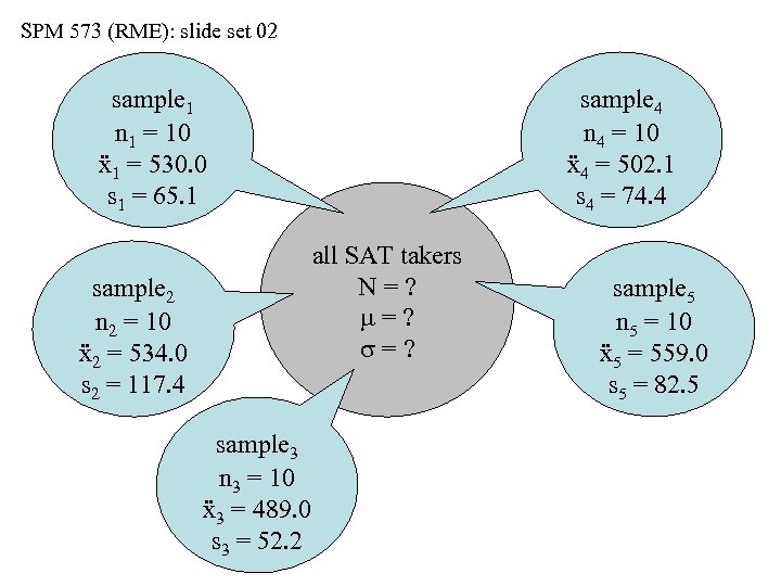 SPM 573 (RME): slide set 02 sample 1 n 1 = 10 ẍ1 = 530. 0 s 1 = 65. 1 sample 4 n 4 = 10 ẍ4 = 502. 1 s 4 = 74. 4 all SAT takers N=? m=? s=? sample 2 n 2 = 10 ẍ2 = 534. 0 s 2 = 117. 4 sample 3 n 3 = 10 ẍ3 = 489. 0 s 3 = 52. 2 sample 5 n 5 = 10 ẍ5 = 559. 0 s 5 = 82. 5
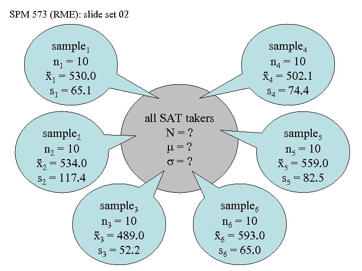 SPM 573 (RME): slide set 02 sample 1 n 1 = 10 ẍ1 = 530. 0 s 1 = 65. 1 sample 4 n 4 = 10 ẍ4 = 502. 1 s 4 = 74. 4 all SAT takers N=? m=? s=? sample 2 n 2 = 10 ẍ2 = 534. 0 s 2 = 117. 4 sample 3 n 3 = 10 ẍ3 = 489. 0 s 3 = 52. 2 sample 5 n 5 = 10 ẍ5 = 559. 0 s 5 = 82. 5 sample 6 n 6 = 10 ẍ6 = 593. 0 s 6 = 65. 0
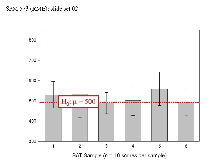
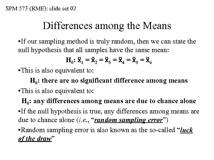 SPM 573 (RME): slide set 02 Differences among the Means • If our sampling method is truly random, then we can state the null hypothesis that all samples have the same mean: H 0: ẍ1 = ẍ2 = ẍ3 = ẍ4 = ẍ5 = ẍ6 • This is also equivalent to: H 0: there are no significant difference among means • This is also equivalent to: H 0: any differences among means are due to chance alone • If the null hypothesis is true, any differences among means are due to chance alone (i. e. , “random sampling error”) • Random sampling error is also known as the so-called “luck of the draw”
 SPM 573 (RME): slide set 02
 SPM 573 (RME): slide set 02
 SPM 573 (RME): slide set 02 H 0: m = 500
 SPM 573 (RME): slide set 02 Box-plot:
 SPM 573 (RME): slide set 02 Box-plot: top outlier 90 th-percentile 75 th-percentile 50 th-percentile 25 th-percentile 10 th-percentile bottom outlier
 SPM 573 (RME): slide set 02 Same Data – Different Interpretations
 SPM 573 (RME): slide set 02
 SPM 573 (RME): slide set 02 m
 SPM 573 (RME): slide set 02 m m 1 s 68. 26%
 SPM 573 (RME): slide set 02 m m 1 s 68. 26% m 2 s 95. 45%
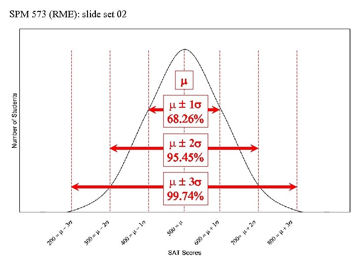 SPM 573 (RME): slide set 02 m m 1 s 68. 26% m 2 s 95. 45% m 3 s 99. 74%
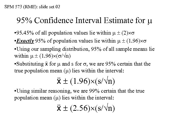 SPM 573 (RME): slide set 02 95% Confidence Interval Estimate for m • 95. 45% of all population values lie within m (2) s • Exactly 95% of population values lie within m (1. 96) s • Using our sampling distribution, 95% of all sample means lie within m (1. 96) (s/ n) • Substituting ẍ for m and s for s, we are 95% certain that the true population mean (m) lies within the interval: ẍ (1. 96) (s/ n) • Using similar reasoning, we are 99% certain that the true population mean (m) lies within the interval: ẍ (2. 56) (s/ n)
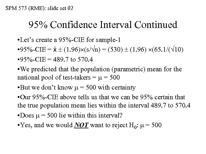 SPM 573 (RME): slide set 02 95% Confidence Interval Continued • Let’s create a 95%-CIE for sample-1 • 95%-CIE = ẍ (1. 96) (s/ n) = (530) (1. 96) (65. 1/( 10) • 95%-CIE = 489. 7 to 570. 4 • We predicted that the population (parametric) mean for the national pool of test-takers = m = 500 • But we don’t know m = 500 with certainty • Our 95%-CIE above tells us that we can be 95% certain that the true population mean lies within the interval 489. 7 to 570. 4 • Does m = 500 lie within this interval? • Yes, and we would NOT want to reject H 0: m = 500
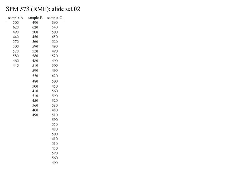
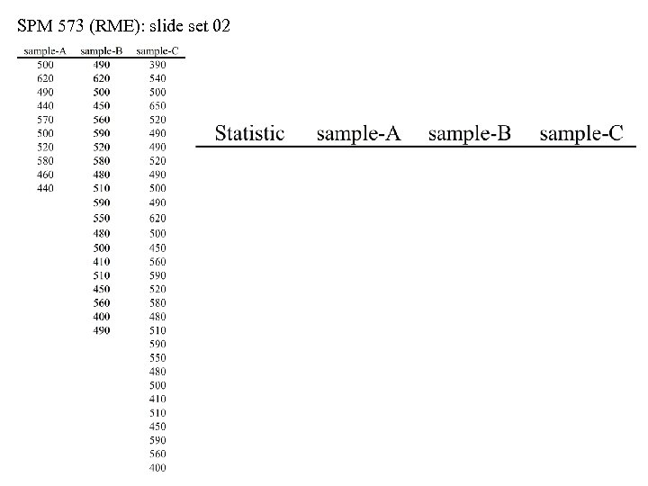
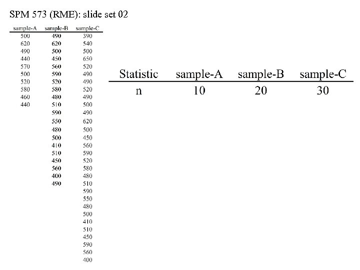
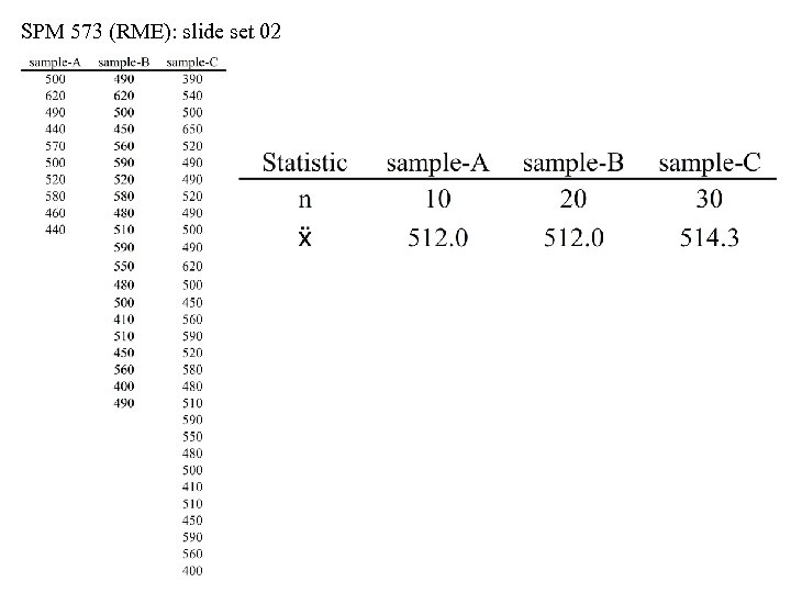
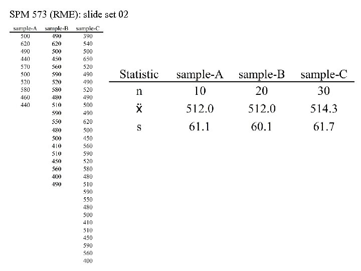
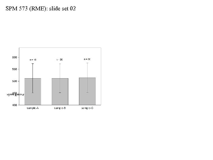
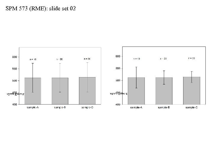
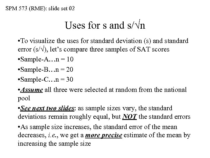 SPM 573 (RME): slide set 02 Uses for s and s/ n • To visualize the uses for standard deviation (s) and standard error (s/ ), let’s compare three samples of SAT scores • Sample-A…n = 10 • Sample-B…n = 20 • Sample-C…n = 30 • Assume all three were selected at random from the national pool • See next two slides: as sample sizes vary, the standard deviations remain roughly equal, but NOT the standard errors • As sample size increases, the standard error of the mean decreases, i. e. , we get a more precise estimate of the mean by increasing the sample size
 SPM 573 (RME): slide set 02
 SPM 573 (RME): slide set 02
 SPM 573 (RME): slide set 02
 SPM 573 (RME): slide set 02
 SPM 573 (RME): slide set 02
 SPM 573 (RME): slide set 02
 SPM 573 (RME): slide set 02
 SPM 573 (RME): slide set 02
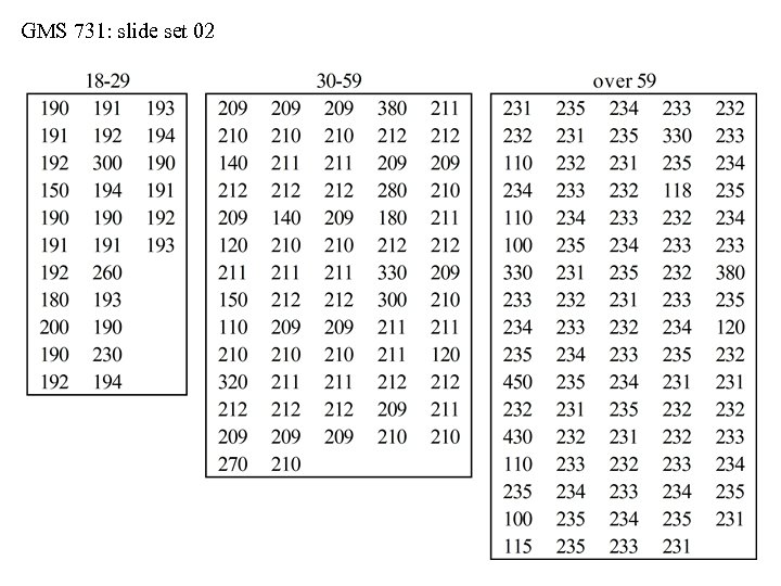
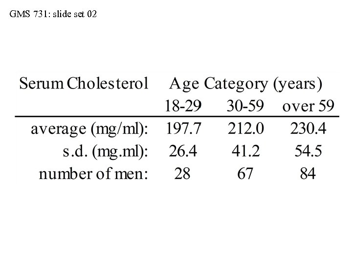
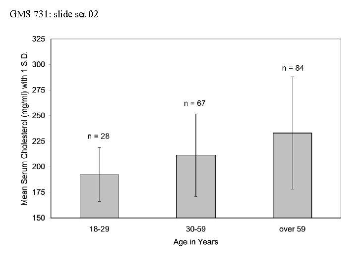
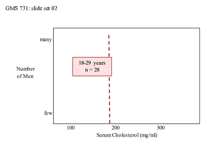
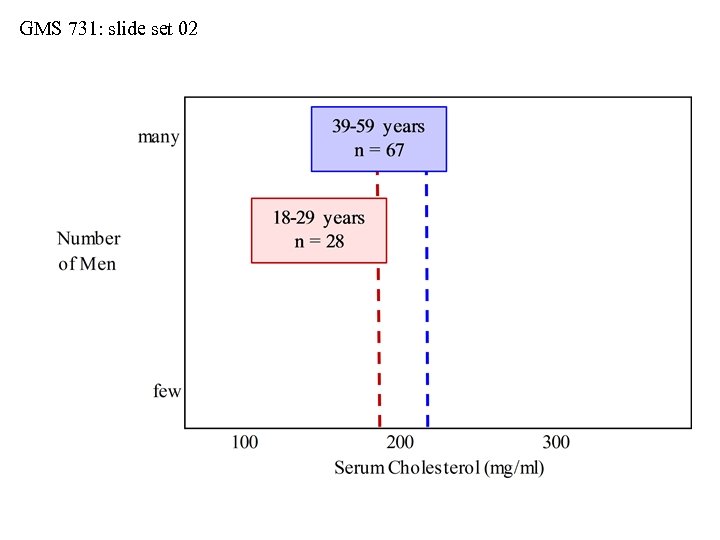
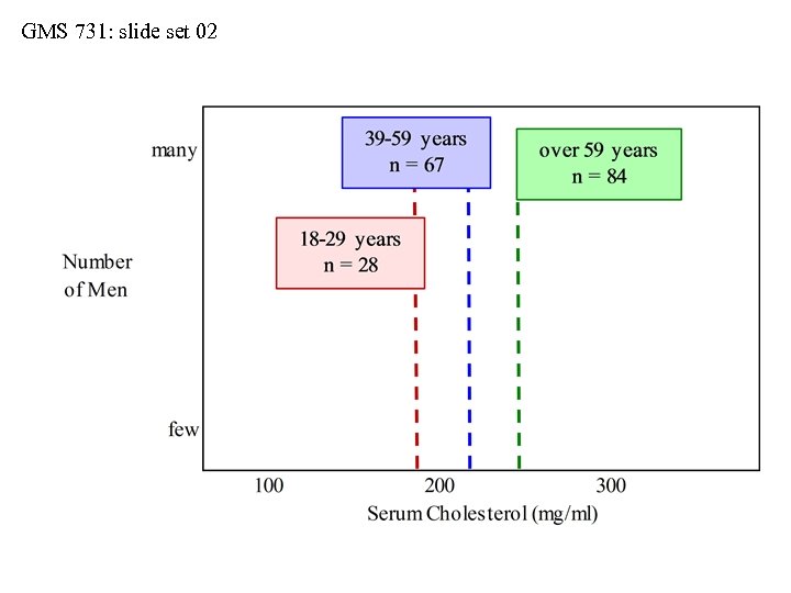
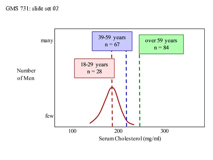
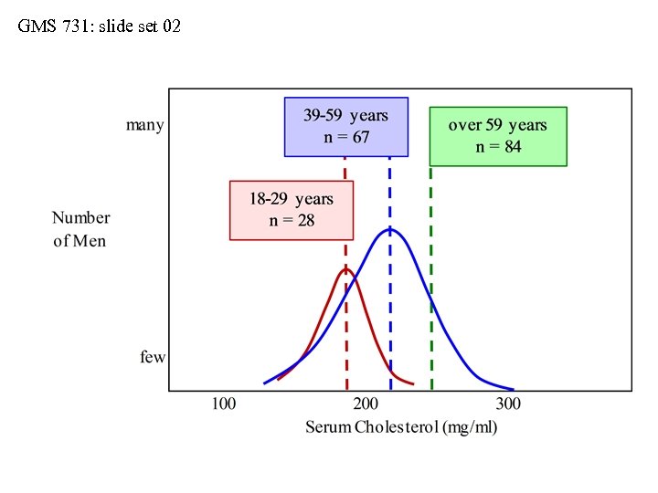
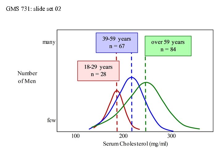
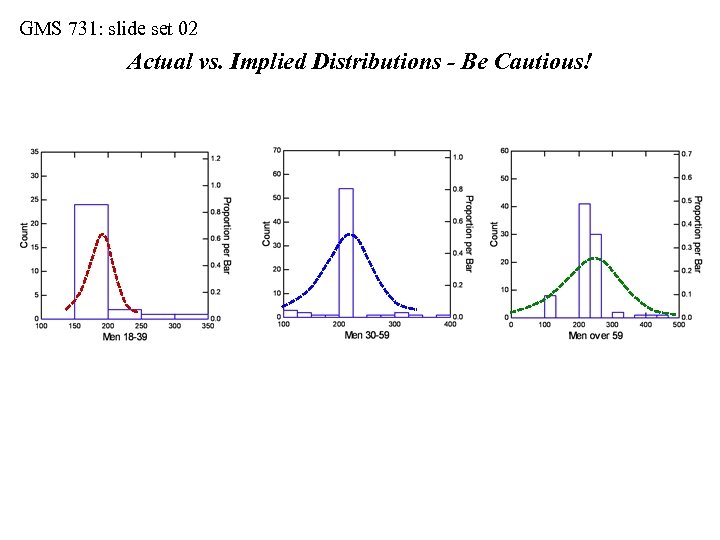
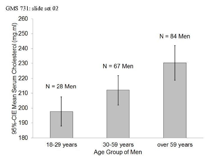
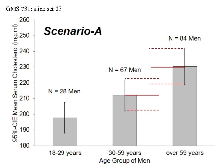
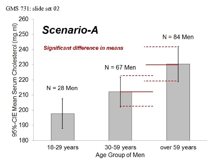
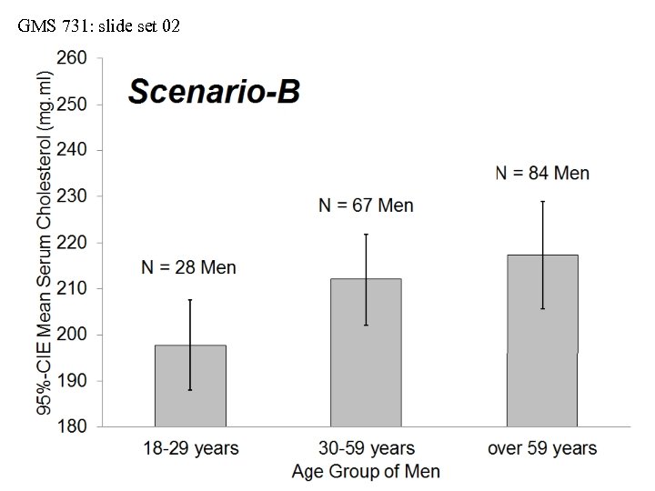
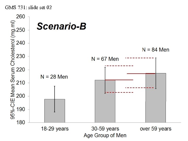
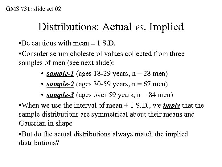 GMS 731: slide set 02 Distributions: Actual vs. Implied • Be cautious with mean ± 1 S. D. • Consider serum cholesterol values collected from three samples of men (see next slide): • sample-1 (ages 18 -29 years, n = 28 men) • sample-2 (ages 30 -59 years, n = 67 men) • sample-3 (ages over 59 years, n = 84 men) • When we use the interval of mean ± 1 S. D. , we imply that the sample distributions are symmetrical about their means and Gaussian in shape • But do the actual distributions always match the implied distributions?
 GMS 731: slide set 02
 GMS 731: slide set 02
 GMS 731: slide set 02
 GMS 731: slide set 02
 GMS 731: slide set 02
 GMS 731: slide set 02
 GMS 731: slide set 02
 GMS 731: slide set 02
 GMS 731: slide set 02
 GMS 731: slide set 02
 GMS 731: slide set 02 Actual vs. Implied Distributions - Be Cautious!
 GMS 731: slide set 02
 GMS 731: slide set 02
 GMS 731: slide set 02 Significant difference in means
 GMS 731: slide set 02
 GMS 731: slide set 02
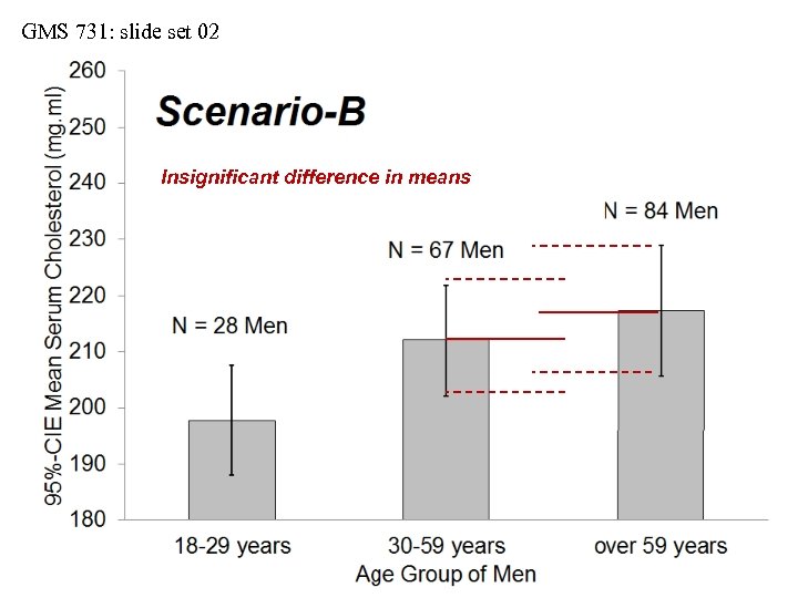 GMS 731: slide set 02 Insignificant difference in means


