
Splatting Jian Huang, CS 594, Spring 2002 This


- Размер: 3.6 Mегабайта
- Количество слайдов: 80
Описание презентации Splatting Jian Huang, CS 594, Spring 2002 This по слайдам
Splatting Jian Huang, CS 594, Spring 2002 This set of slides reference slides made by Ohio State University alumuni over the past several years.
Volumetric Ray Integration color opacity object ( color , opacity )1.
Splatting • Lee Westover — Vis 1989; SIGGRAPH 1990 • Object order method • Front-To-Back or Back-To-Front • Original method — fast, poor quality • Many many improvements since then! – Crawfis’ 93: textured splats – Swan’ 96, Mueller’ 97: anti-aliasing – Mueller’ 98: image-aligned sheet-based splatting – Mueller’ 99: post-classified splatting – Huang’ 00: new splat primitive: Fast. Splats
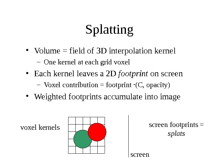
Splatting • Volume = field of 3 D interpolation kernel – One kernel at each grid voxel • Each kernel leaves a 2 D footprint on screen – Voxel contribution = footprint ·(C, opacity) • Weighted footprints accumulate into image voxel kernels screen footprints = splats screen
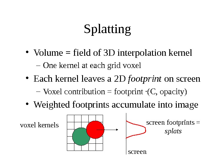
Splatting • Volume = field of 3 D interpolation kernel – One kernel at each grid voxel • Each kernel leaves a 2 D footprint on screen – Voxel contribution = footprint ·(C, opacity) • Weighted footprints accumulate into image voxel kernels screen footprints = splats screen
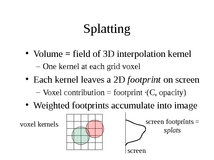
Splatting • Volume = field of 3 D interpolation kernel – One kernel at each grid voxel • Each kernel leaves a 2 D footprint on screen – Voxel contribution = footprint ·(C, opacity) • Weighted footprints accumulate into image voxel kernels screen footprints = splats screen
Splatting • Volume = field of 3 D interpolation kernel – One kernel at each grid voxel • Each kernel leaves a 2 D footprint on screen – Voxel contribution = footprint ·(C, opacity) • Weighted footprints accumulate into image voxel kernels screen footprints = splats screen
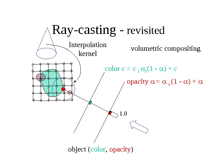
Ray-casting — revisited color c = c s s (1 — ) + c opacity = s (1 — ) + 1. 0 object ( color , opacity )volumetric compositing. Interpolation kernel
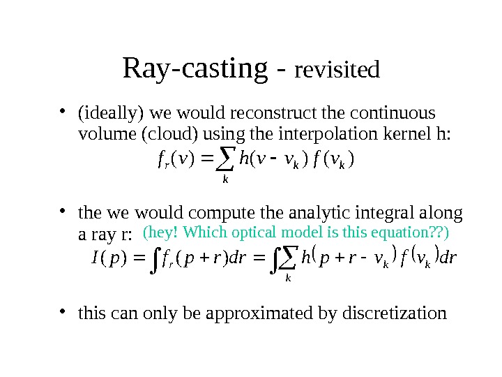
Ray-casting — revisited • (ideally) we would reconstruct the continuous volume (cloud) using the interpolation kernel h: • the we would compute the analytic integral along a ray r: • this can only be approximated by discretization k kkrdrvfvrphdrrpfp. I)()( k kkrvfvvhvf)()()( (hey! Which optical model is this equation? ? )
Splatting — principal idea • This last equation • can be rewritten in the following way: k kkdrvfvrphp. I)( k kkdrvrphvfp. I)( Splatting Kernel or “Splat” Which can be computed analytically : known as footprint dzzyxhyx , , ), (Splat
Footprint Extent Approximate the 3 D kernel (h(x, y, z))extent by a sphere
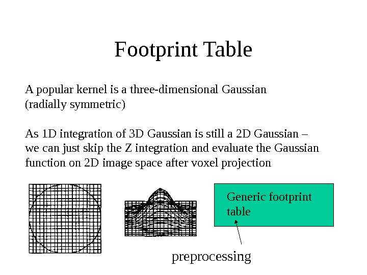
Footprint Table A popular kernel is a three-dimensional Gaussian (radially symmetric) As 1 D integration of 3 D Gaussian is still a 2 D Gaussian – we can just skip the Z integration and evaluate the Gaussian function on 2 D image space after voxel projection Generic footprint table preprocessing
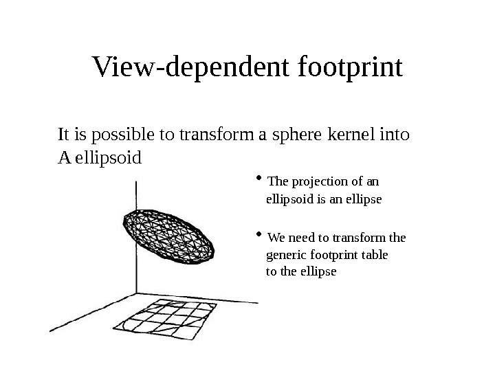
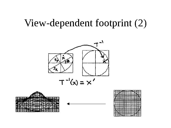
View-dependent footprint It is possible to transform a sphere kernel into A ellipsoid • The projection of an ellipsoid is an ellipse • We need to transform the generic footprint table to the ellipse
View-dependent footprint (2)
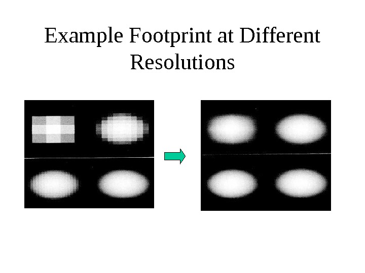
Example Footprint at Different Resolutions
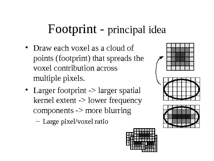
Footprint — principal idea • Draw each voxel as a cloud of points (footprint) that spreads the voxel contribution across multiple pixels. • Larger footprint -> larger spatial kernel extent -> lower frequency components -> more blurring – Large pixel/voxel ratio
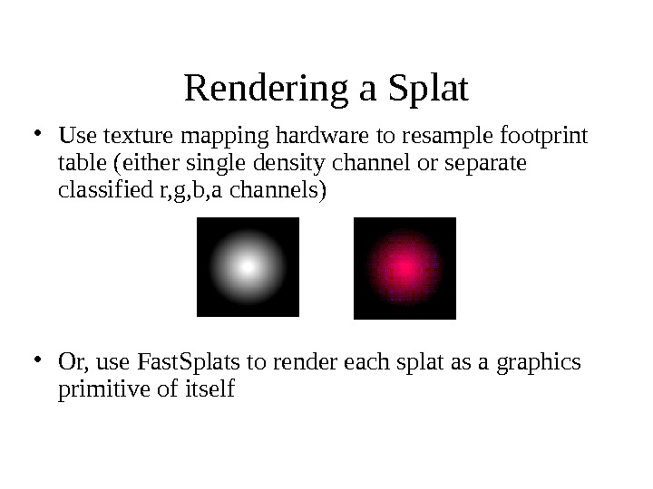
Rendering a Splat • Use texture mapping hardware to resample footprint table (either single density channel or separate classified r, g, b, a channels) • Or, use Fast. Splats to render each splat as a graphics primitive of itself
Splatting — efficiency • “ footprint” — splatted (integrated) kernel • if interpolation kernel is isotropic (spherical) then its footprint is independent of the view point (for orthographic viewing) • for perspective — footprint can be approximated with an ellipse • Hence, for common cases, we can pre-integrate it (efficient!) • for perspective projection, to approximate, we have to compute the orientation of the ellipse
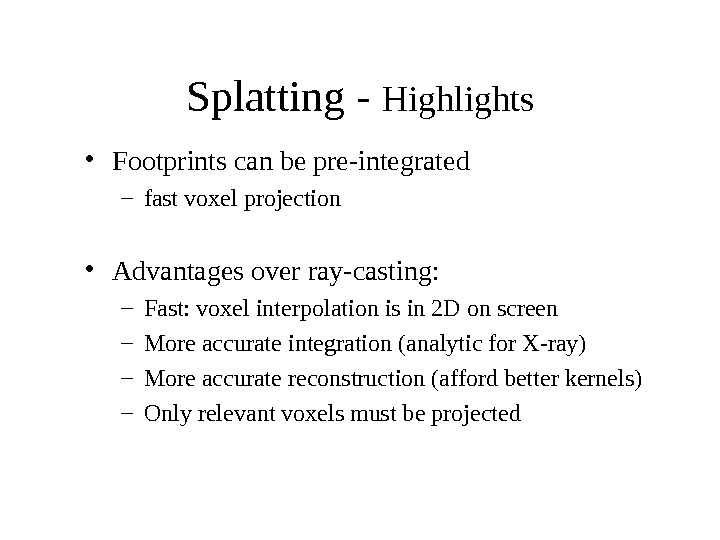
Splatting — Highlights • Footprints can be pre-integrated – fast voxel projection • Advantages over ray-casting: – Fast: voxel interpolation is in 2 D on screen – More accurate integration (analytic for X-ray) – More accurate reconstruction (afford better kernels) – Only relevant voxels must be projected
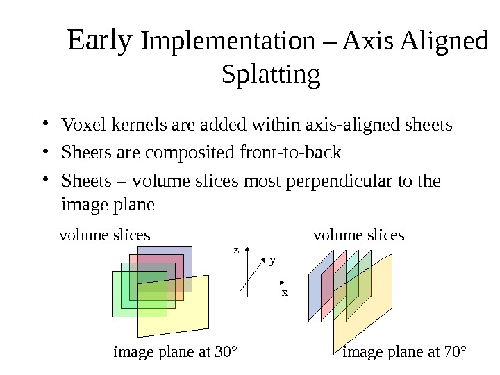
Early Implementation – Axis Aligned Splatting • Voxel kernels are added within axis-aligned sheets • Sheets are composited front-to-back • Sheets = volume slices most perpendicular to the image plane at 70° image plane at 30° volume slices xyz volume slices
Early Implementation – Axis Aligned Splatting sheet buffer compositing buffer volume slices image plane • Volume
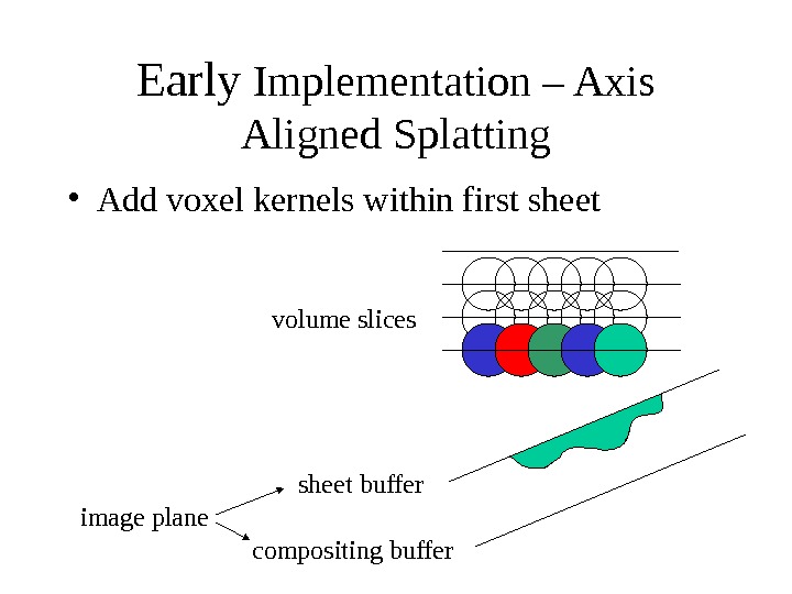
Early Implementation – Axis Aligned Splatting sheet buffer compositing buffer volume slices image plane • Add voxel kernels within first sheet
Early Implementation – Axis Aligned Splatting sheet buffer compositing buffer volume slices image plane • Transfer to compositing buffer
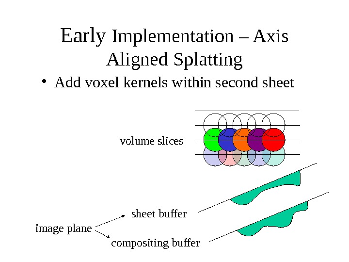
Early Implementation – Axis Aligned Splatting sheet buffer compositing buffer volume slices image plane • Add voxel kernels within second sheet
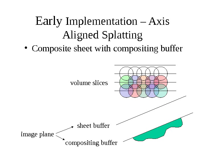
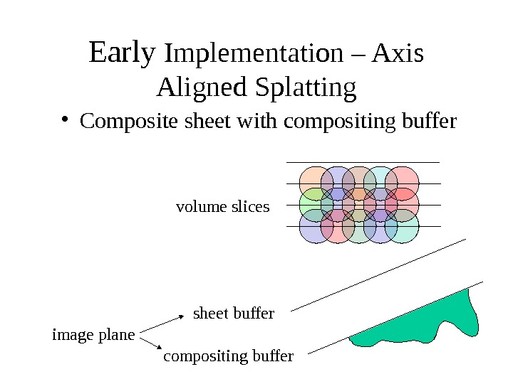
Early Implementation – Axis Aligned Splatting sheet buffer compositing buffer volume slices image plane • Composite sheet with compositing buffer
Early Implementation – Axis Aligned Splatting sheet buffer compositing buffer volume slices image plane • Add voxel kernels within third sheet
Early Implementation – Axis Aligned Splatting sheet buffer compositing buffer volume slices image plane • Composite sheet with compositing buffer
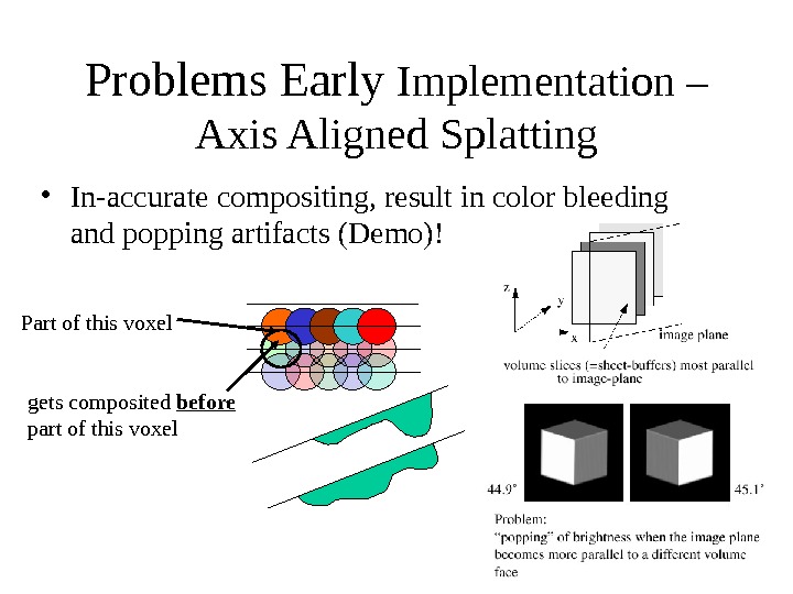
What Doesn’t Work? • Mathematically, the early splatting methods only work for X-ray type of rendering, where voxel ordering is not important – Bad approximation for other types of optical models • Object ordering is important in volume rendering, front objects hide back objects – need to composite splats in proper order, else we get bleeding of background objects into the image (color bleeding!) • Axis- aligned approach add all splats that fall within a volume slice most parallel to the image plane, composite these sheets in front- to- back order – Incorrect accumulating on axis-aligned face cause popping • A better approximation with Riemann sum is to use the image-aligned sheet-based approach
Problems Early Implementation – Axis Aligned Splatting • In-accurate compositing, result in color bleeding and popping artifacts (Demo)! Part of this voxel gets composited before part of this voxel
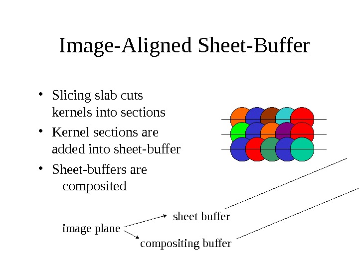
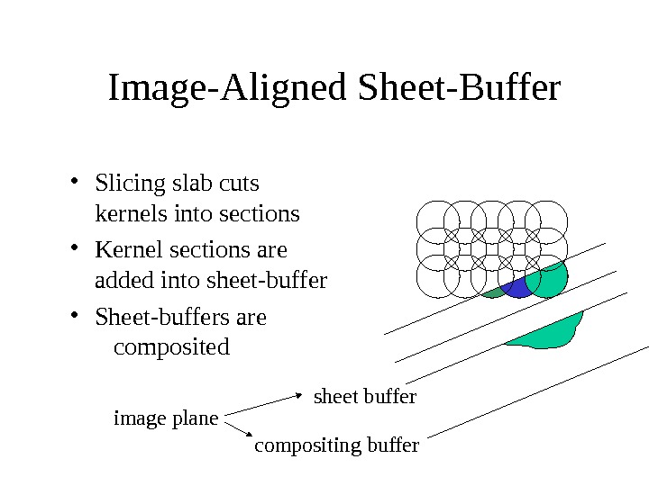
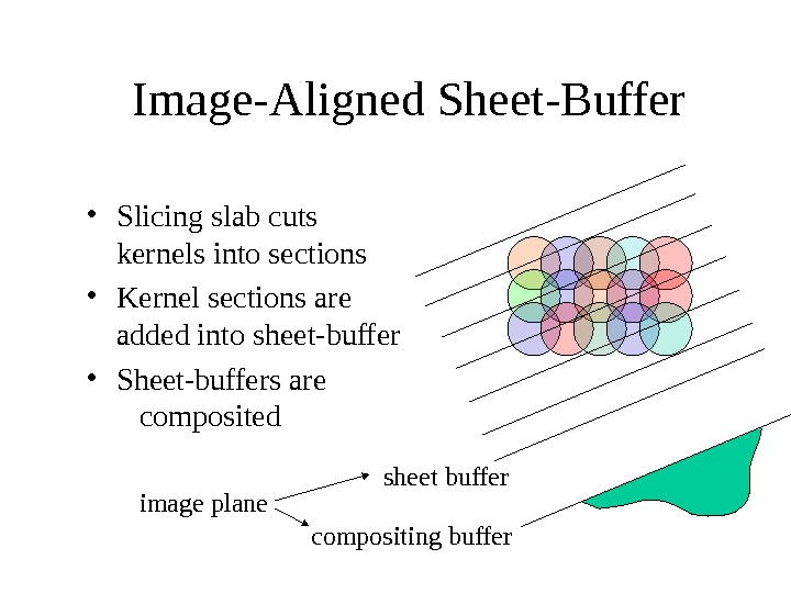
Image-Aligned Sheet-Buffer sheet buffer compositing buffer • Slicing slab cuts kernels into sections • Kernel sections are added into sheet-buffer • Sheet-buffers are composited image plane
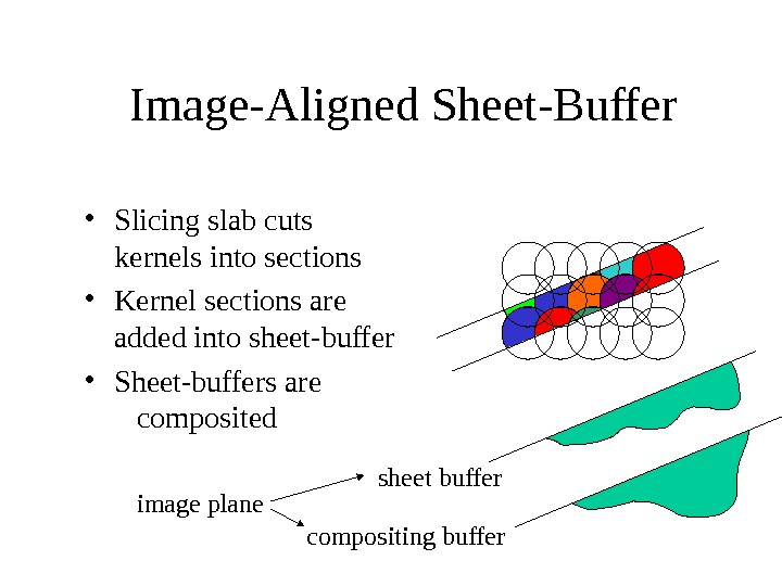
Image-Aligned Sheet-Buffer sheet buffer compositing buffer • Slicing slab cuts kernels into sections • Kernel sections are added into sheet-buffer • Sheet-buffers are composited image plane
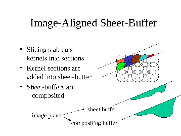
Image-Aligned Sheet-Buffer sheet buffer compositing buffer • Slicing slab cuts kernels into sections • Kernel sections are added into sheet-buffer • Sheet-buffers are composited image plane
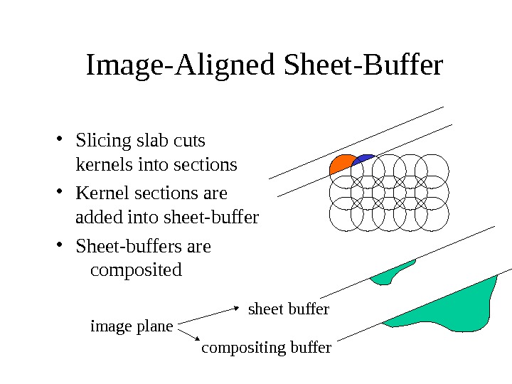
Image-Aligned Sheet-Buffer sheet buffer compositing buffer • Slicing slab cuts kernels into sections • Kernel sections are added into sheet-buffer • Sheet-buffers are composited image plane
Image-Aligned Sheet-Buffer sheet buffer compositing buffer • Slicing slab cuts kernels into sections • Kernel sections are added into sheet-buffer • Sheet-buffers are composited image plane
Image-Aligned Sheet-Buffer sheet buffer compositing buffer • Slicing slab cuts kernels into sections • Kernel sections are added into sheet-buffer • Sheet-buffers are composited image plane
Image-Aligned Sheet-Buffer sheet buffer compositing buffer • Slicing slab cuts kernels into sections • Kernel sections are added into sheet-buffer • Sheet-buffers are composited image plane
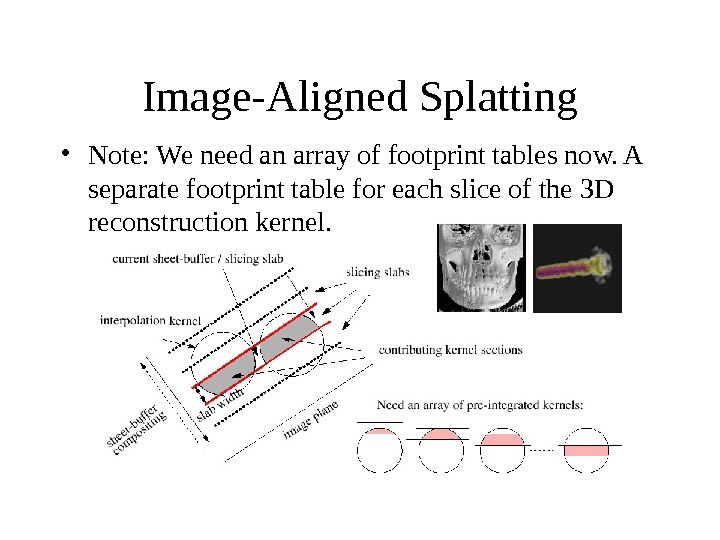
Image-Aligned Splatting • Note: We need an array of footprint tables now. A separate footprint table for each slice of the 3 D reconstruction kernel.
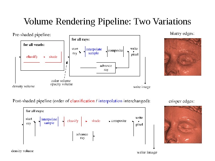
Volume Rendering Pipeline: Two Variations
Volume Rendering Pipeline: Two Variations
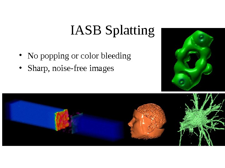
IASB Splatting • No popping or color bleeding • Sharp, noise-free images
Occlusion Culling • A voxel is only visible if the volume material in front is not opaque occluded voxel: does not pass visibility test wall of occluding voxels occlusion map = opacity image screen
Visibility Test Based on SAT of Occlusion Buffer opacity threshold occlusion map. Do not project Project opacity < threshold opacity = 0 • Compute occlusion map after each sheet • Cull both individual voxel and voxel sets with a summed area table of occlusion map
Occlusion Culling • Build a summed area table (SAT) from the opacity buffer • To test whether a rectangular region is opaque or not, check the four corners • Can cull voxel sets directly
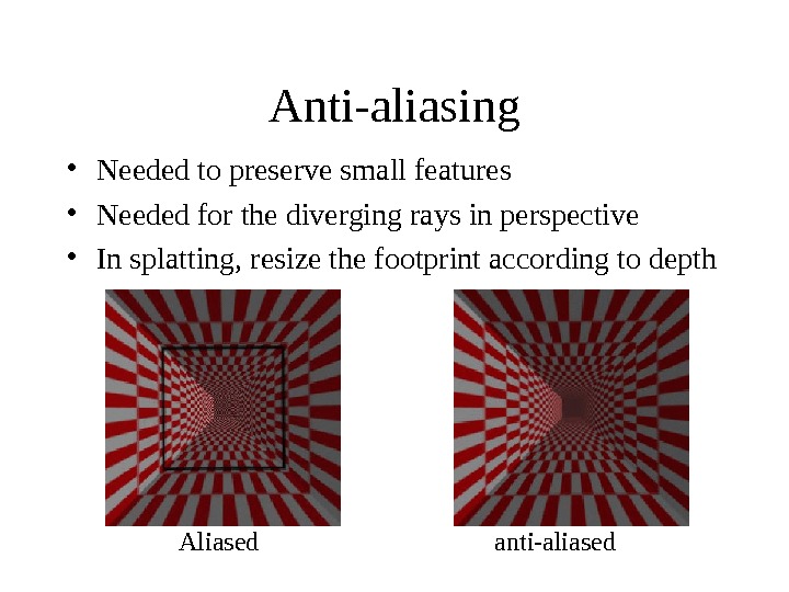
Anti-aliasing • Needed to preserve small features • Needed for the diverging rays in perspective • In splatting, resize the footprint according to depth Aliased anti-aliased
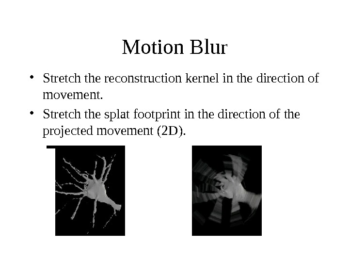
Motion Blur • Stretch the reconstruction kernel in the direction of movement. • Stretch the splat footprint in the direction of the projected movement (2 D).
Camera Depth-of-Field • Two possible approaches: – Low-pass filter the splats – Low-pass filter the sheets Plain with Depth-of-Field
Procedural Textures • Easily done with pre-coloring • Per-pixel
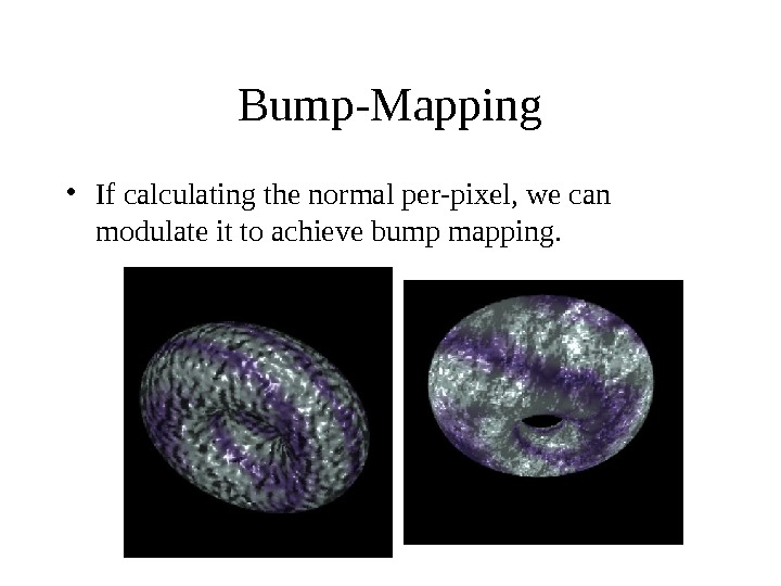
Bump-Mapping • If calculating the normal per-pixel, we can modulate it to achieve bump mapping.
Per-pixel Classification • Per-pixel classification can be based on gray scale, position, gradient, or. . . 7. 25 sec 9. 41 sec (procedural) 7. 99 sec
Scan-Converting A Splat • Scan-convert an arbitrary-size radially symmetric 2 D function centered at arbitrary position – circular or elliptical • Texture mapping hardware is not the solution • We want a hardware accelerated splat or point primitive
Fast Splats Fast. Splat • We desire – fast scan conversion – minimum or controllable errors – compact storage – simple integer operation
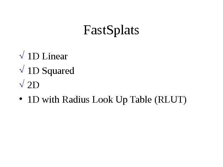
Fast. Splats 1 D Linear 1 D Squared 2 D 1 D with Radius Look Up Table (RLUT)
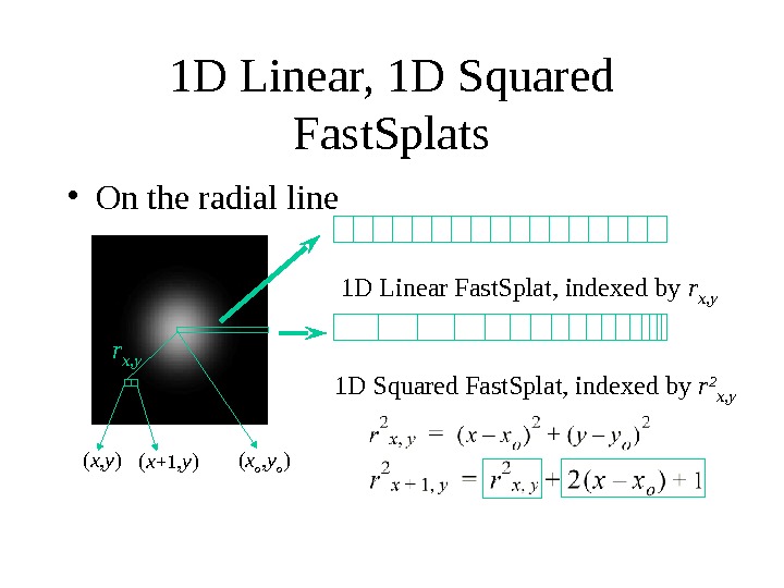
1 D Linear, 1 D Squared Fast. Splats • On the radial line 1 D Linear Fast. Splat, indexed by r x, y 1 D Squared Fast. Splat, indexed by r 2 x, y ( x, y ) ( x +1 , y )r x, y ( x o , y o )
1 D Squared Fast. Splat (Elliptical) • For elliptical kernels, if we define a canonical radius: • The incremental scan-conversion still works at the same low cost
Fast. Splats 1 D Linear 1 D Squared 2 D • 1 D with Radius Look Up Table (RLUT)
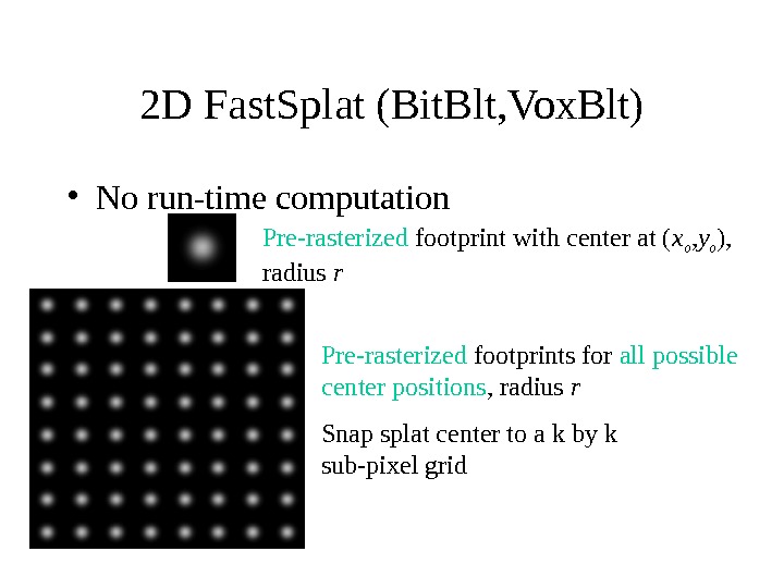
2 D Fast. Splat (Bit. Blt, Vox. Blt) • No run-time computation Pre-rasterized footprint with center at ( x o , y o ), radius r Pre-rasterized footprints for all possible center positions , radius r Snap splat center to a k by k sub-pixel grid
2 D Fast. Splats • No run-time computation Pre-rasterized footprints for all possible center positions , for all possible radii Snap splat center to a k by k sub-pixel grid Allow for a set of radius values
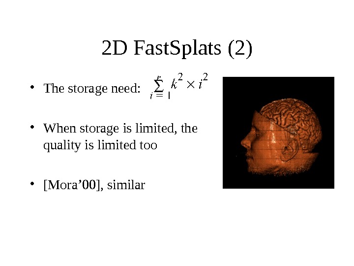
2 D Fast. Splats (2) • The storage need: • When storage is limited, the quality is limited too • [Mora’ 00], similar
Fast. Splats 1 D Linear 1 D Squared 2 D • 1 D with Radius Look Up Table (RLUT)
1 D RLUT Fast. Splat • For hardware, we need finer parallelism than scan-line
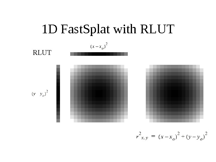
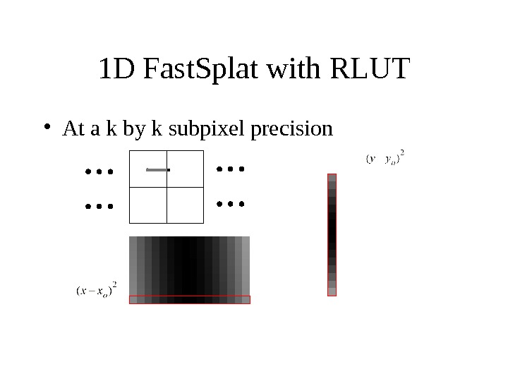
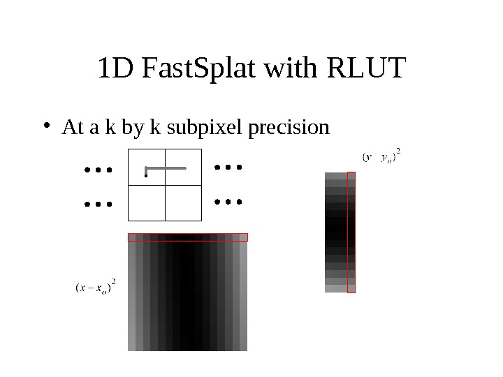
1 D Fast. Splat with RLUT
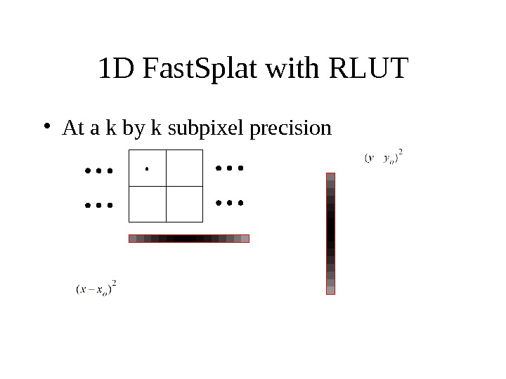
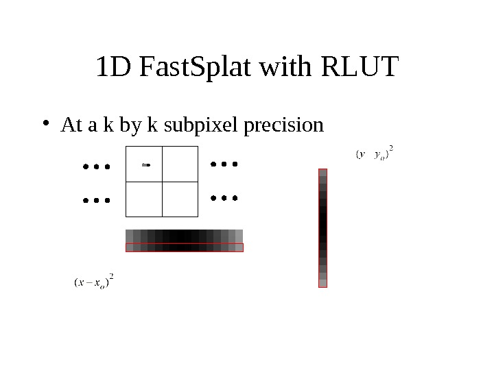
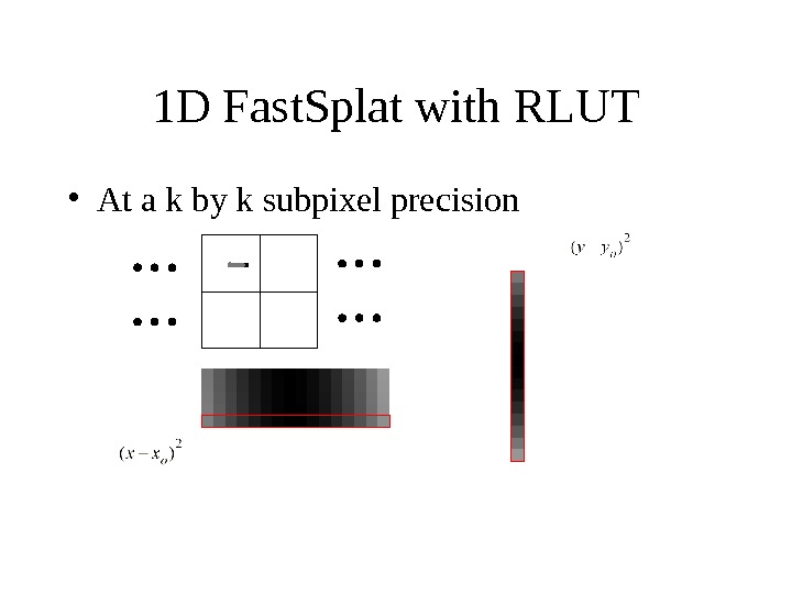
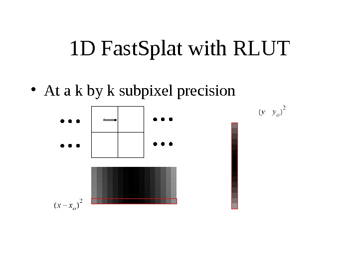
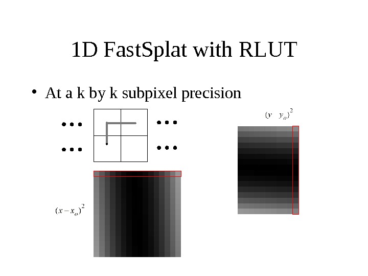
1 D Fast. Splat with RLUT • At a k by k subpixel precision
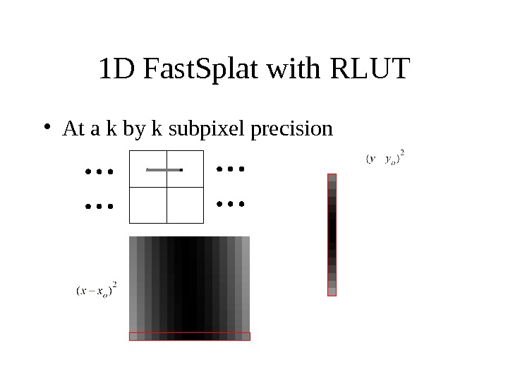
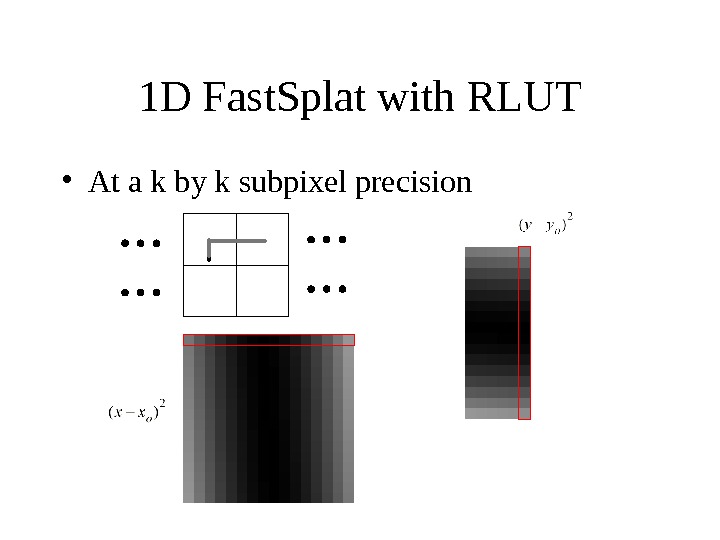
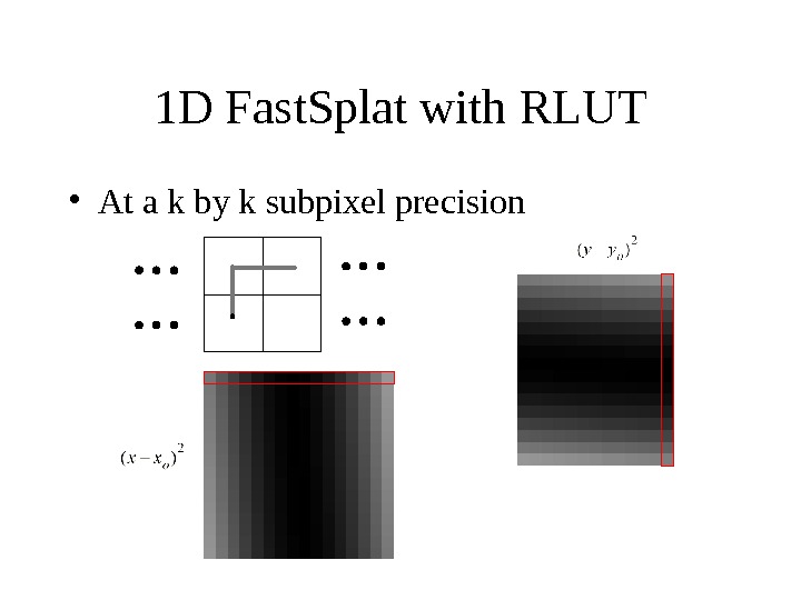
1 D Fast. Splat with RLUT • At a k by k subpixel precision
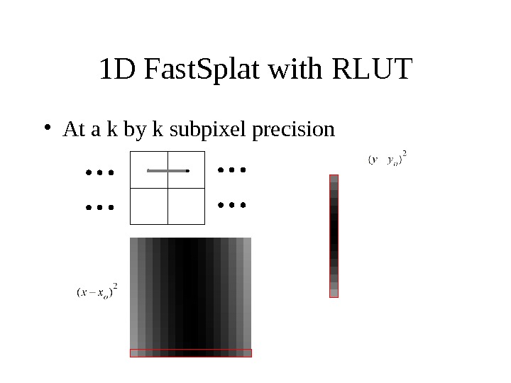
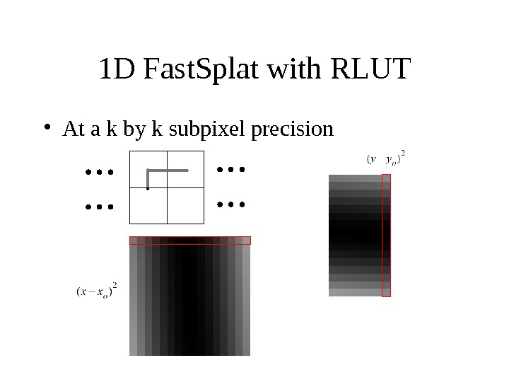
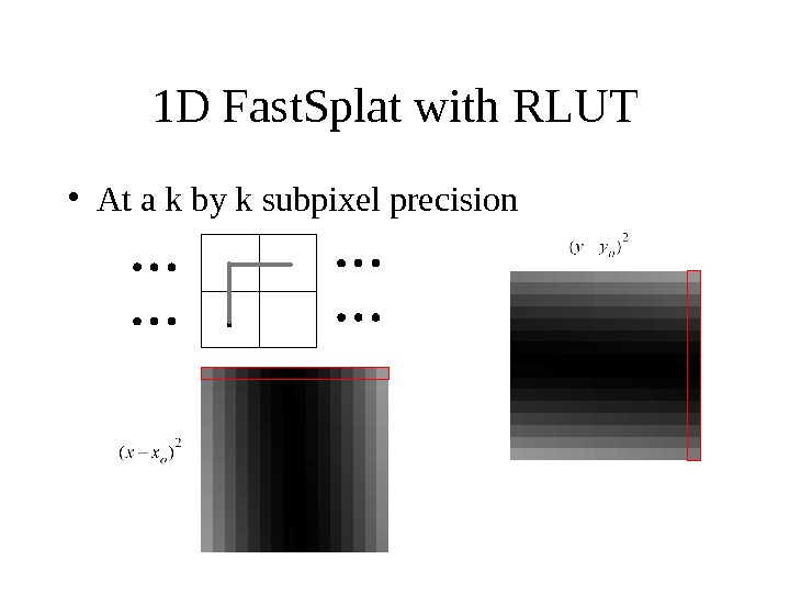
1 D Fast. Splat with RLUT • At a k by k subpixel precision
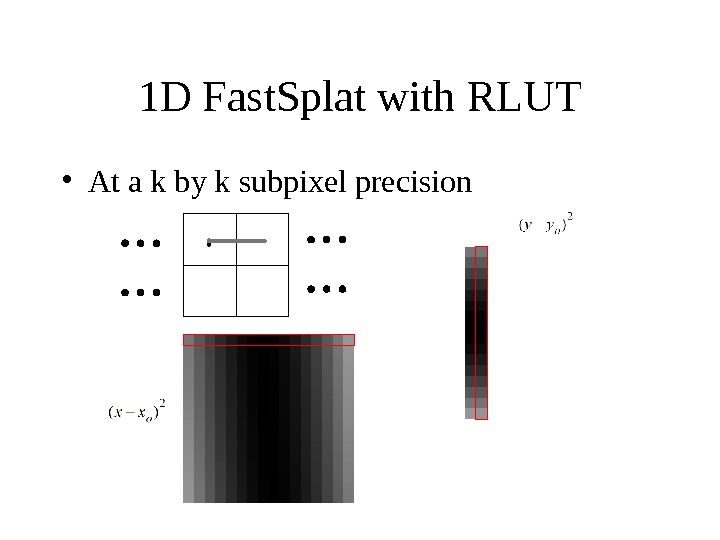
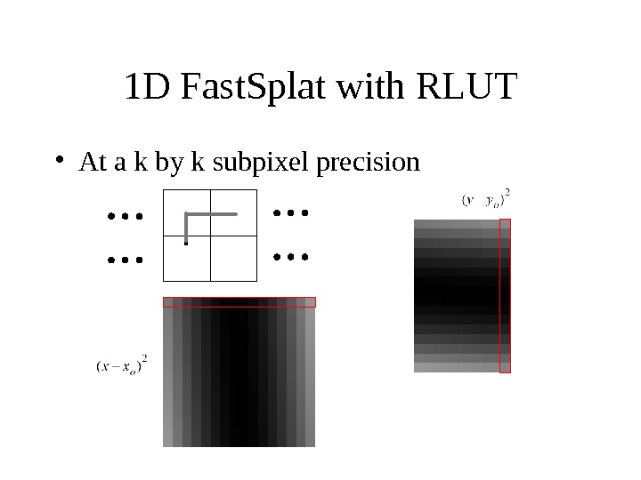
1 D Fast. Splat with RLUT • At a k by k subpixel precision
1 D Fast. Splat with RLUT • At a k by k subpixel precision
1 D Fast. Splat with RLUT • At a k by k subpixel precision
1 D Fast. Splat with RLUT • At a k by k subpixel precision
1 D Fast. Splat with RLUT • At a k by k subpixel precision
1 D Fast. Splat with RLUT • At a k by k subpixel precision
1 D Fast. Splat with RLUT • At a k by k subpixel precision
1 D Fast. Splat with RLUT • At a k by k subpixel precision
1 D Fast. Splat with RLUT • At a k by k subpixel precision
1 D Fast. Splat with RLUT • At a k by k subpixel precision
1 D Fast. Splat with RLUT • At a k by k subpixel precision
1 D Fast. Splat with RLUT • At a k by k subpixel precision
1 D Fast. Splat with RLUT • At a k by k subpixel precision
1 D Fast. Splat with RLUT • k by k subpixel precision
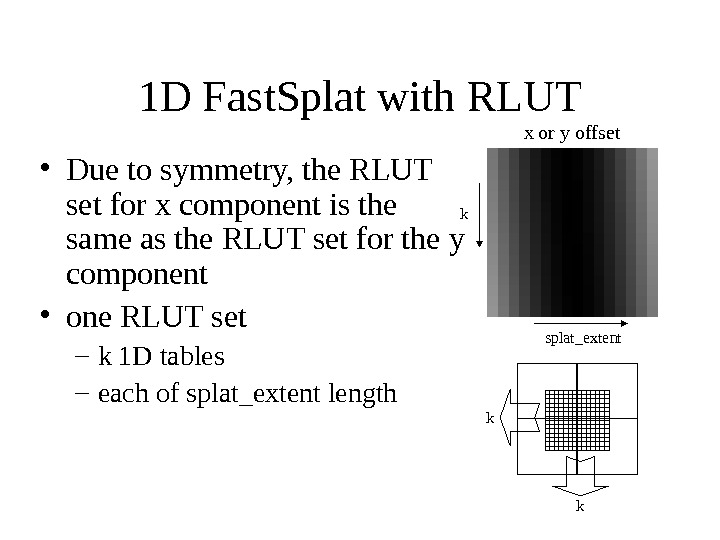
1 D Fast. Splat with RLUT • Due to symmetry, the RLUT set for x component is the same as the RLUT set for the y component • one RLUT set – k 1 D tables – each of splat_extent length x or y offset k splat_extent k k
Comparisons Among the Fast. Splats • 1 D Linear: very accurate, compact, slow • 1 D Squared: accurate, compact, fast • 1 D RLUT: accurate, compact, intended for hardware • 2 D Fast. Splat: can be very fast, accurate and compact under constrained conditions