Spending Output Income Spending Aggregate Demand Aggregate Supply

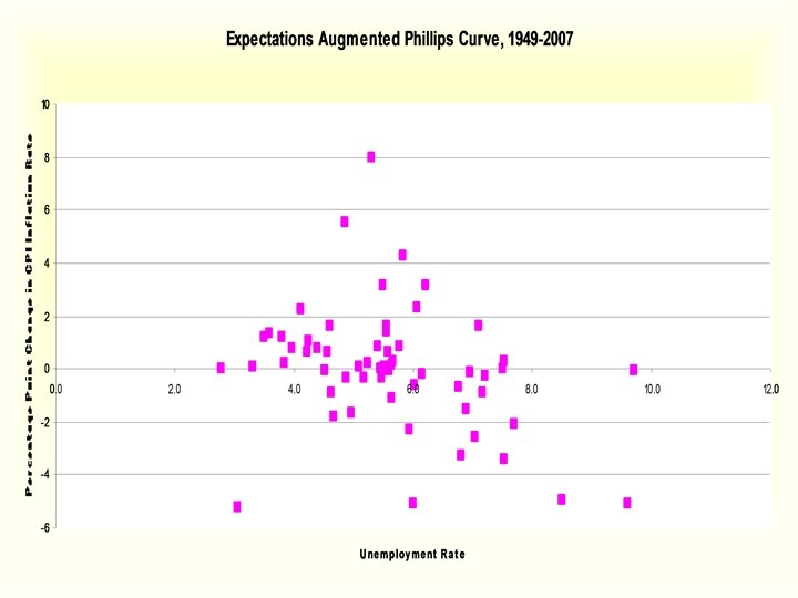
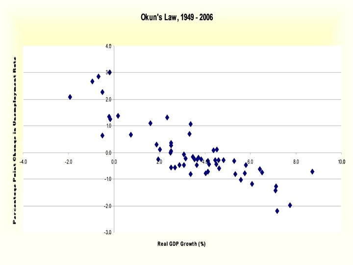
Spending Output Income Spending Aggregate Demand Aggregate Supply Y = C + I + G + NX Why AD slopes downward Why AD might shift Why Short-run AS (SRAS) slopes upward Vertical LRAS Why AS might shift—Recall: Costs Supply “Long-run” (Medium run) AS-AD Equilibrium Expectations Augmented Phillips Curve Okun’s Law Money Supply—Money multiplier Money Demand—Money market equilibrium Response to monetary expansion Response to fiscal expansion Spending multiplier/Crowding out Automatic stabilizers Rules vs. discretion

Spending Output Income Spending n n $GDP: The market value of all final goods and services produced in our economy in a year GDP Deflator (=P): The dollar value of a year’s outputs relative to what it would have been had prices remained constant at base year prices. • In practice, the increase in a year’s prices over the prior year’s (for all the things produced this year – C, I, G, and X) chained to the base year. n Real GDP (= Y): $GDP measured at base year prices Real GDP = $GDP/Price Deflator Y = $GDP/P

Aggregate Demand Aggregate Supply. . . Price Level Aggregate supply Equilibrium price level Aggregate demand 0 Equilibrium output Quantity of Output

The Aggregate Demand Curve u The four components of GDP (Y) contribute to the aggregate demand for goods and services. Y = C + I + G + NX

The Aggregate-Demand Curve. . . Price Level P 1 1. A decrease in the price level. . . P 2 Aggregate demand 0 Y 1 Y 2 2. …increases the quantity of goods and services demanded. Quantity of Output

Why the Aggregate Demand Curve Is Downward Sloping u Price Level and Consumption: u. Wealth Effect …the purchasing power of money balances u Price Level and Investment: u. Interest u Price Rate Effect Level and Net Exports: u. Substitution effect u. The Exchange-Rate Effect via real balances and interest rate

Why the Aggregate Demand Curve Might Shift u Shifts arising from Consumption u. Changes in wealth u. House prices u. Stock prices u Shifts arising from Investment u. Responses to interest rate u. New technologies u. Animal Spirits u Shifts arising from Government Purchases u Shifts arising from Net Exports

The Aggregate Supply Curve u In the long run, the aggregatesupply curve is vertical. u In the short run, the aggregatesupply curve is upward sloping.

The Short-Run Aggregate Supply Curve. . . Price Level Short-run aggregate supply P 1 1. A decrease in the price level P 2 0 2. reduces the quantity of goods and services supplied in the short run. Y 2 Y 1 Quantity of Output

Why the Aggregate Supply Curve Slopes Upward in the Short Run u Sticky u High – wages Profit Up when Prices Up output Low Unemployment Wages Up Prices Up

The Long-Run Aggregate. Supply Curve. . . Price Level P 1 Long-run aggregate supply 2. …does not affect the quantity of goods and services supplied in the long run. P 2 1. A change in the price level… 0 Natural rate of output Quantity of Output

Why the Aggregate Supply Curve Might Shift: Recall: Supply reflects costs u Shifts arising from Labor u. Higher wages higher costs given output can/will only be supplied at higher price u Shifts arising from Capital u. Increase in capacity increase in supply u Shifts arising from Natural Resources u. Increase in resource price increased costs u Shifts arising from Technology. u Shifts arising from the Expected Price Level.

The Long-Run Equilibrium Price Level Equilibrium price 0 Short-run aggregate supply Long-run aggregate supply A Natural rate of output Aggregate demand Quantity of Output

A Contraction in Aggregate Demand. . . Price Level 2. …causes output to fall in the short run… Long-run aggregate supply Short-run aggregate supply, AS 1 AS 2 3. …but over time, the short-run aggregate-supply curve shifts… A P 1 P 2 B P 3 1. A decrease in aggregate demand… C AD 2 0 Y 2 Y 1 Aggregate demand, AD 1 4. …and output returns to its natural rate. Quantity of Output

Money Supply Means of Payment: Currency + Demand Deposits = Money multiplier x Monetary Base = Money multiplier x (Currency + Reserves) u. The money supply is controlled by the Fed through: u Open-market operations u Changing reserve requirements u Changing the discount rate u The public’s willingness to deposit money in banks and bank willingness to lend matter as well

Money Demand u The opportunity cost of holding money is the interest that could be earned on interest-earning assets—bonds u An increase in the interest rate raises the opportunity cost of holding money. u As a result, the quantity of money demanded is reduced

Harcourt, Inc. items and derived items copyright © 2001 by Harcourt, Inc. Equilibrium in the Money Market. . . Interest Rate Money supply r 1 Equilibrium interest rate r 2 0 Money demand d M 1 Quantity fixed by the Fed d M 2 Quantity of Money

The Money Market and the Slope of the Aggregate Demand Curve. . . (a) The Money Market Interest Rate (b) The Aggregate Demand Curve Price Level Money supply 2. …increases the demand for money… r 2 1. An increase in the price level… P 2 Money demand at price level P 2, MD 2 Aggregate demand P 1 r 1 Money demand at price level P 1, MD 1 0 Quantity fixed by the Fed 3. …which increases the equilibrium rate… Quantity of Money 0 Y 2 Y 1 Quantity of Output 4. …which in turn reduces the quantity of goods and services demanded.

Harcourt, Inc. items and derived items copyright © 2001 by Harcourt, Inc. A Monetary Injection. . . (a) The Money Market Interest Rate Money supply, MS 1 MS 2 (b) The Aggregate-Demand Curve 3. …which increases the quantity of goods and services demanded at a given price level. Price Level 1. When the Fed increases the money supply… P r 1 r 2 AD 2 Aggregate demand, AD 1 0 2. …the equilibrium interest rate falls… Quantity of Money 0 Y 1 Y 2 Quantity of Output

Changes in Government Purchases u. Macroeconomic effects from change in government purchases: u. The multiplier effect u. The crowding-out effect

The Multiplier Effect. . . Price Level 2. …but the multiplier effect can amplify the shift in aggregate demand. $20 billion AD 3 1. An increase in government purchases of $20 billion initially increases aggregate demand by $20 billion… 0 AD 2 Aggregate demand, AD 1 Quantity of Output

Formula for the Simpler Spending Multiplier = 1/(1 - MPC) u MPC u It is the marginal propensity to consume is the fraction of extra income that households consume rather than save. u The greater the MPC, the more total output (Y), income and spending results from an initial increase in spending

The Crowding-Out Effect. . . (a) The Money Market Interest Rate Price Level Money supply r 2 (b) The Shift in Aggregate Demand 2. …the increase in spending increases money demand… $20 billion AD 2 r 1 MD 2 AD 3 Aggregate demand, AD 1 Money demand, MD 1 0 4. …which in turn partly offsets the initial increase in aggregate demand. Quantity fixed by the Fed Quantity of Money 3. …which increases the equilibrium interest rate… 0 Quantity of Output 1. When an increase in government purchases increases aggregate demand…

Automatic Stabilizers u. Automatic stabilizers are changes in fiscal policy that stimulate aggregate demand when the economy goes into a recession without policymakers having to take any deliberate action. u. Automatic stabilizers include the tax system and some forms of government spending.

The Case for Active Stabilization Policy The Employment Act has two implications: u The government should avoid being the cause of economic fluctuations. u The government should respond to changes in the private economy in order to stabilize aggregate demand, e. g. , the Bush tax rebate and Obama’s stimulus package u. Obama insisted that only government could “break the vicious cycles that are crippling our economy, ” prevent “the catastrophic failure of financial institutions, ” restart the flow of credit and restore the regulations needed to prevent such a crisis in the future. January 8, 2009

The Case Against Active Stabilization Policy u Active monetary and fiscal policies may destabilize the economy. u Monetary and fiscal policies affect the economy with a substantial lag. u They suggest the economy should be left to deal with the short-run fluctuations on its own. u. Avoid monetary mischief