Spatial Preprocessing John Ashburner john fil ion ucl ac

Spatial Preprocessing John Ashburner john@fil. ion. ucl. ac. uk z Smoothing z Rigid registration z Spatial normalisation With slides by Chloe Hutton and Jesper Andersson

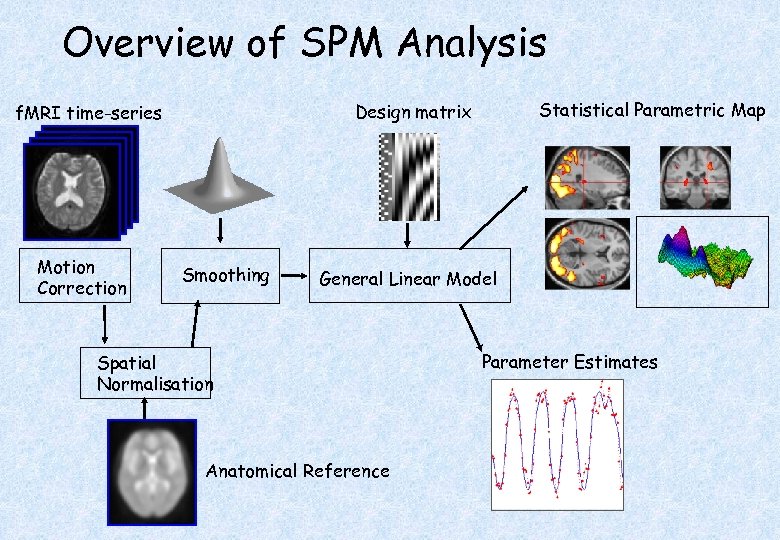
Overview of SPM Analysis Motion Correction Statistical Parametric Map Design matrix f. MRI time-series Smoothing General Linear Model Spatial Normalisation Anatomical Reference Parameter Estimates

Contents z. Smoothing z. Rigid registration z. Spatial normalisation

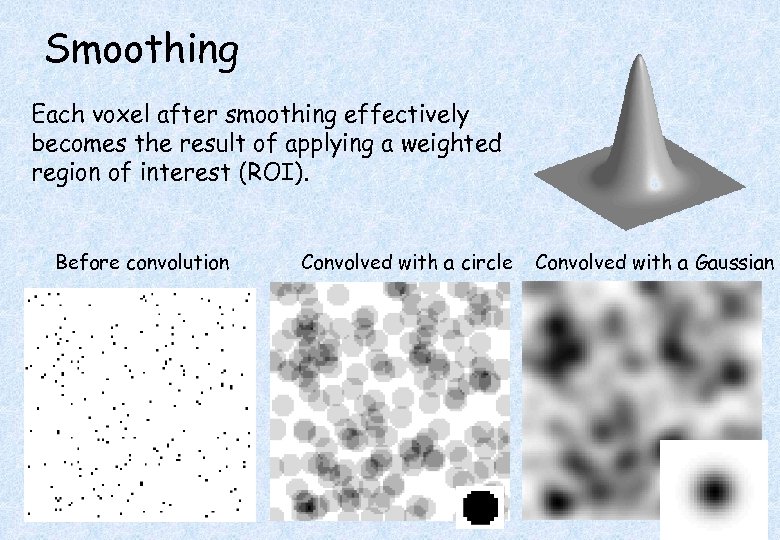
Smoothing Each voxel after smoothing effectively becomes the result of applying a weighted region of interest (ROI). Before convolution Convolved with a circle Convolved with a Gaussian

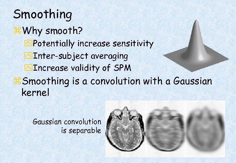
Smoothing z. Why smooth? y. Potentially increase sensitivity y. Inter-subject averaging y. Increase validity of SPM z. Smoothing is a convolution with a Gaussian kernel Gaussian convolution is separable

Contents z. Smoothing z. Rigid registration y. Rigid-body transforms y. Optimisation & objective functions y. Interpolation z. Spatial normalisation

Within-subject Registration z. Assumes there is no shape change, and motion is rigid-body z. Used by [realign] and [coregister] functions z. The steps are: z. Registration - i. e. Optimising the parameters that describe a rigid body transformation between the source and reference images z. Transformation - i. e. Re-sampling according to the determined transformation

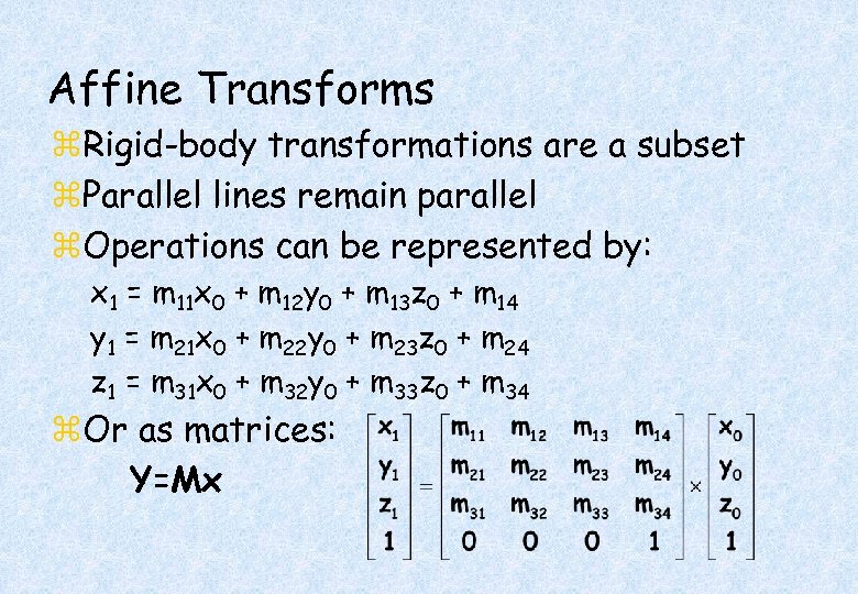
Affine Transforms z. Rigid-body transformations are a subset z. Parallel lines remain parallel z. Operations can be represented by: x 1 = m 11 x 0 + m 12 y 0 + m 13 z 0 + m 14 y 1 = m 21 x 0 + m 22 y 0 + m 23 z 0 + m 24 z 1 = m 31 x 0 + m 32 y 0 + m 33 z 0 + m 34 z. Or as matrices: Y=Mx

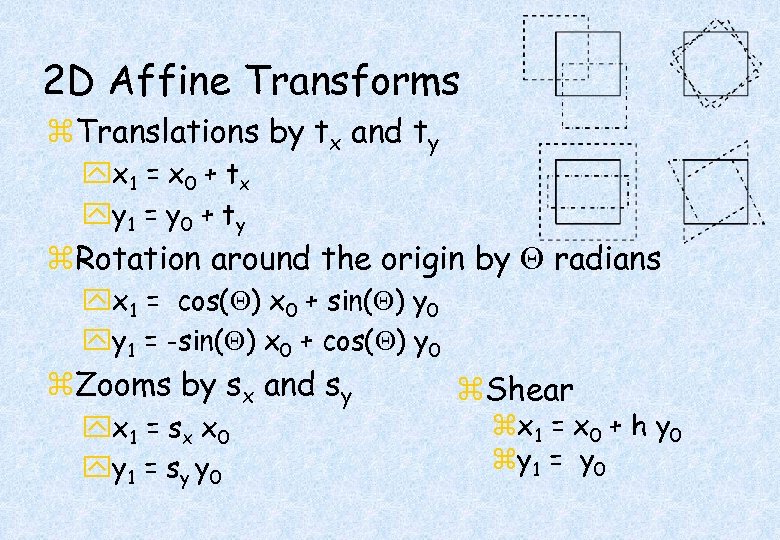
2 D Affine Transforms z. Translations by tx and ty yx 1 = x 0 + t x yy 1 = y 0 + t y z. Rotation around the origin by radians yx 1 = cos( ) x 0 + sin( ) y 0 yy 1 = -sin( ) x 0 + cos( ) y 0 z. Zooms by sx and sy yx 1 = s x x 0 yy 1 = s y y 0 z. Shear zx 1 = x 0 + h y 0 zy 1 = y 0

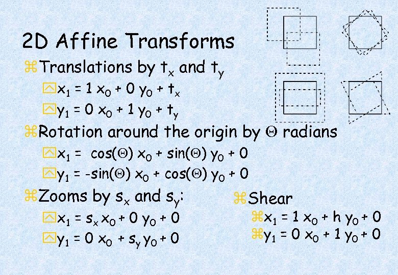
2 D Affine Transforms z. Translations by tx and ty yx 1 = 1 x 0 + 0 y 0 + t x yy 1 = 0 x 0 + 1 y 0 + t y z. Rotation around the origin by radians yx 1 = cos( ) x 0 + sin( ) y 0 + 0 yy 1 = -sin( ) x 0 + cos( ) y 0 + 0 z. Zooms by sx and sy: yx 1 = s x x 0 + 0 yy 1 = 0 x 0 + s y y 0 + 0 z. Shear zx 1 = 1 x 0 + h y 0 + 0 zy 1 = 0 x 0 + 1 y 0 + 0

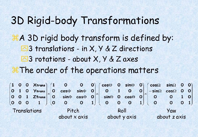
3 D Rigid-body Transformations z. A 3 D rigid body transform is defined by: y 3 translations - in X, Y & Z directions y 3 rotations - about X, Y & Z axes z. The order of the operations matters Translations Pitch about x axis Roll about y axis Yaw about z axis

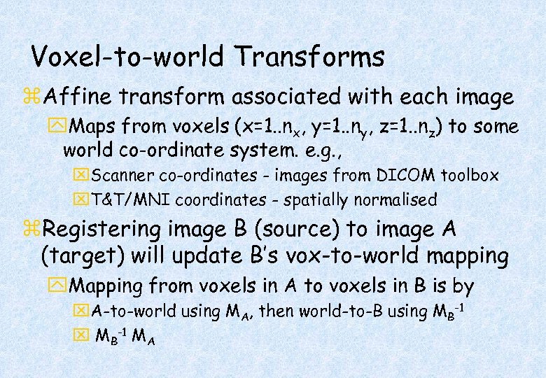
Voxel-to-world Transforms z. Affine transform associated with each image y. Maps from voxels (x=1. . nx, y=1. . ny, z=1. . nz) to some world co-ordinate system. e. g. , x. Scanner co-ordinates - images from DICOM toolbox x. T&T/MNI coordinates - spatially normalised z. Registering image B (source) to image A (target) will update B’s vox-to-world mapping y. Mapping from voxels in A to voxels in B is by x. A-to-world using MA, then world-to-B using MB-1 x MB-1 MA

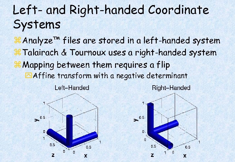
Left- and Right-handed Coordinate Systems z Analyze™ files are stored in a left-handed system z Talairach & Tournoux uses a right-handed system z Mapping between them requires a flip y. Affine transform with a negative determinant

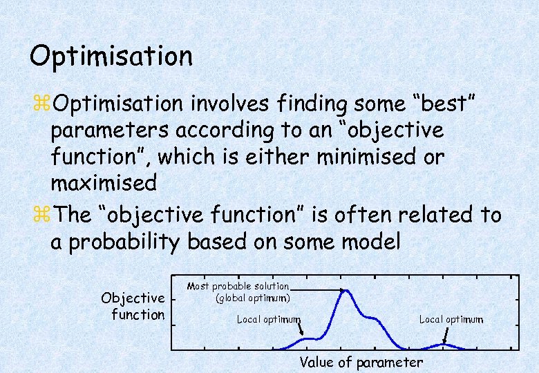
Optimisation z. Optimisation involves finding some “best” parameters according to an “objective function”, which is either minimised or maximised z. The “objective function” is often related to a probability based on some model Objective function Most probable solution (global optimum) Local optimum Value of parameter

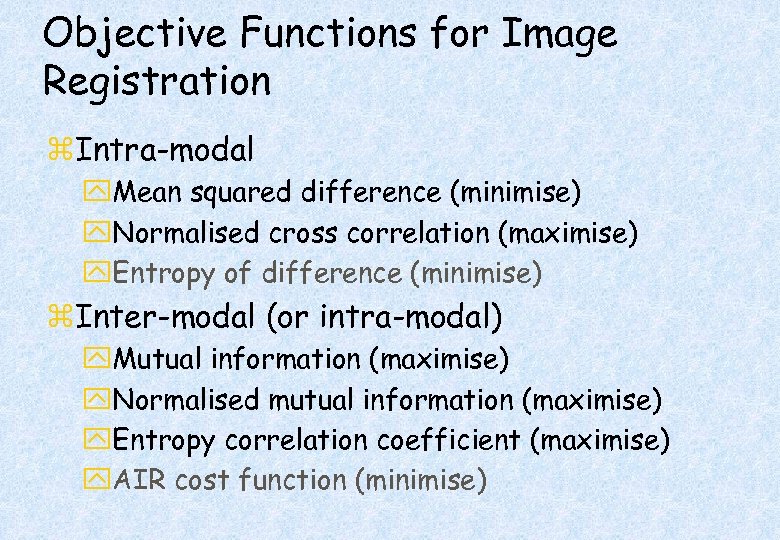
Objective Functions for Image Registration z. Intra-modal y. Mean squared difference (minimise) y. Normalised cross correlation (maximise) y. Entropy of difference (minimise) z. Inter-modal (or intra-modal) y. Mutual information (maximise) y. Normalised mutual information (maximise) y. Entropy correlation coefficient (maximise) y. AIR cost function (minimise)

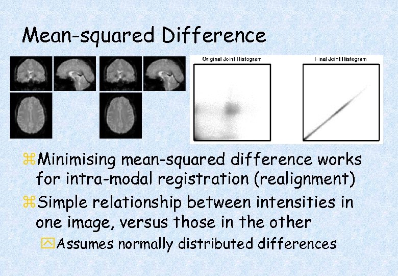
Mean-squared Difference z. Minimising mean-squared difference works for intra-modal registration (realignment) z. Simple relationship between intensities in one image, versus those in the other y. Assumes normally distributed differences

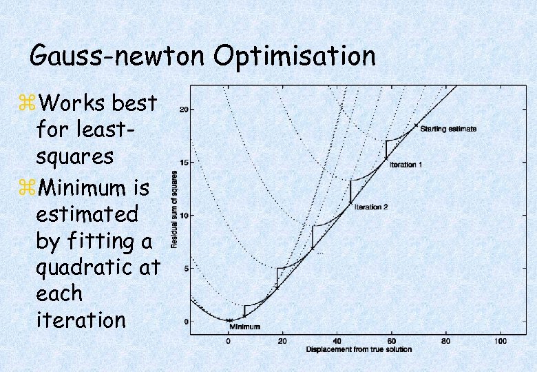
Gauss-newton Optimisation z. Works best for leastsquares z. Minimum is estimated by fitting a quadratic at each iteration

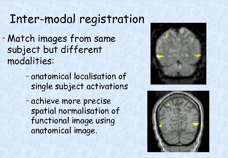
Inter-modal registration • Match images from same subject but different modalities: – anatomical localisation of single subject activations – achieve more precise spatial normalisation of functional image using anatomical image.

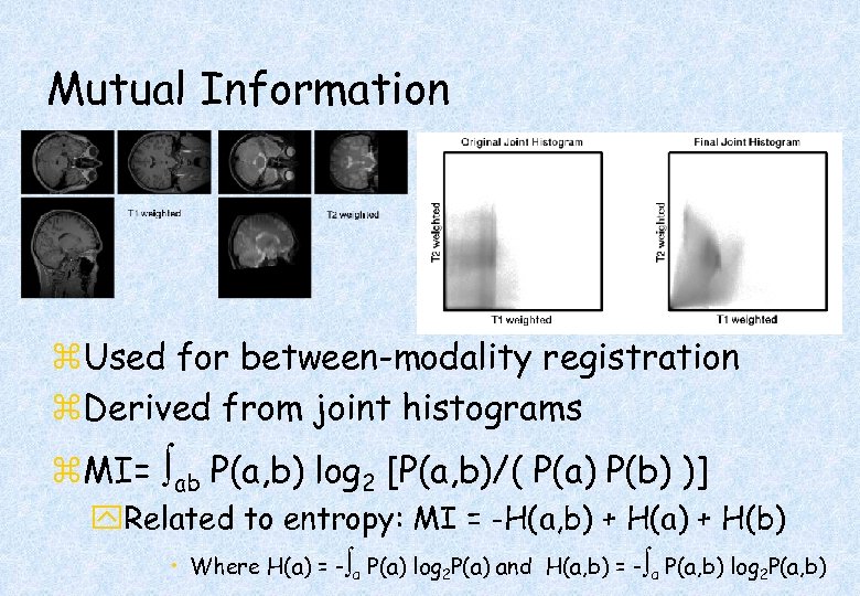
Mutual Information z. Used for between-modality registration z. Derived from joint histograms z. MI= ab P(a, b) log 2 [P(a, b)/( P(a) P(b) )] y. Related to entropy: MI = -H(a, b) + H(a) + H(b) • Where H(a) = - a P(a) log 2 P(a) and H(a, b) = - a P(a, b) log 2 P(a, b)

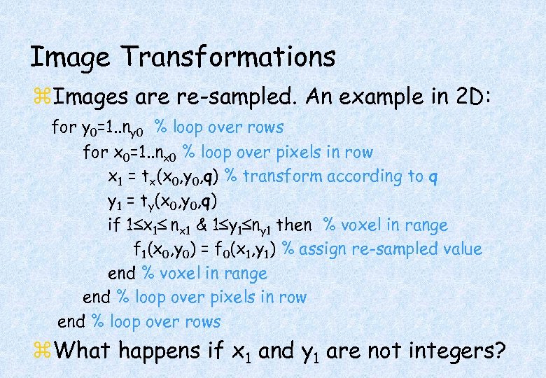
Image Transformations z. Images are re-sampled. An example in 2 D: for y 0=1. . ny 0 % loop over rows for x 0=1. . nx 0 % loop over pixels in row x 1 = tx(x 0, y 0, q) % transform according to q y 1 = ty(x 0, y 0, q) if 1 x 1 nx 1 & 1 y 1 ny 1 then % voxel in range f 1(x 0, y 0) = f 0(x 1, y 1) % assign re-sampled value end % voxel in range end % loop over pixels in row end % loop over rows z. What happens if x 1 and y 1 are not integers?

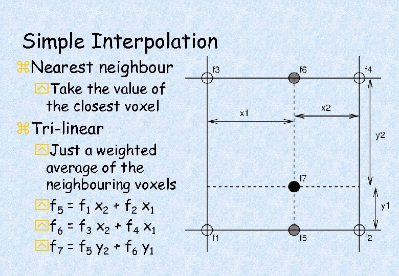
Simple Interpolation z. Nearest neighbour y. Take the value of the closest voxel z. Tri-linear y. Just a weighted average of the neighbouring voxels yf 5 = f 1 x 2 + f 2 x 1 yf 6 = f 3 x 2 + f 4 x 1 yf 7 = f 5 y 2 + f 6 y 1

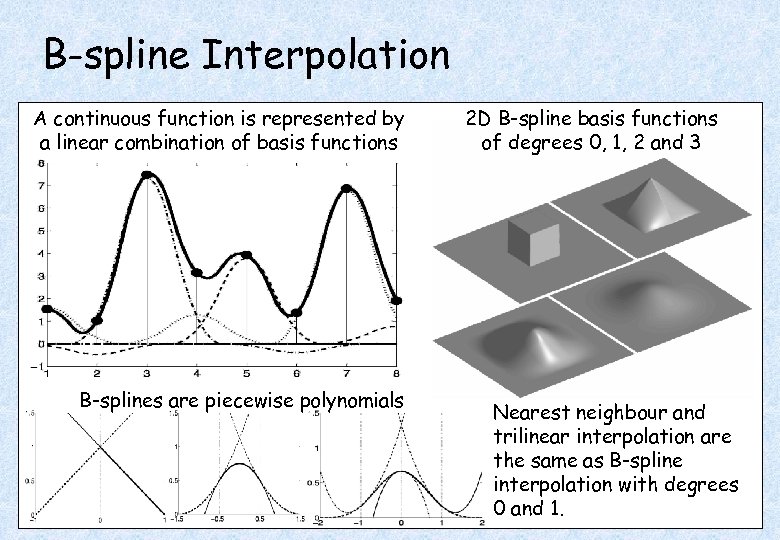
B-spline Interpolation A continuous function is represented by a linear combination of basis functions B-splines are piecewise polynomials 2 D B-spline basis functions of degrees 0, 1, 2 and 3 Nearest neighbour and trilinear interpolation are the same as B-spline interpolation with degrees 0 and 1.

Residual Errors from aligned f. MRI • Re-sampling can introduce interpolation errors – especially tri-linear interpolation • Gaps between slices can cause aliasing artefacts • Slices are not acquired simultaneously – rapid movements not accounted for by rigid body model • Image artefacts may not move according to a rigid body model – image distortion – image dropout – Nyquist ghost • Functions of the estimated motion parameters can be modelled as confounds in subsequent analyses

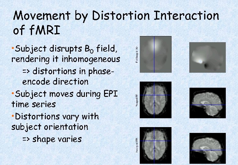
Movement by Distortion Interaction of f. MRI • Subject disrupts B 0 field, rendering it inhomogeneous => distortions in phaseencode direction • Subject moves during EPI time series • Distortions vary with subject orientation => shape varies

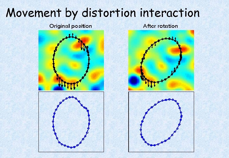
Movement by distortion interaction

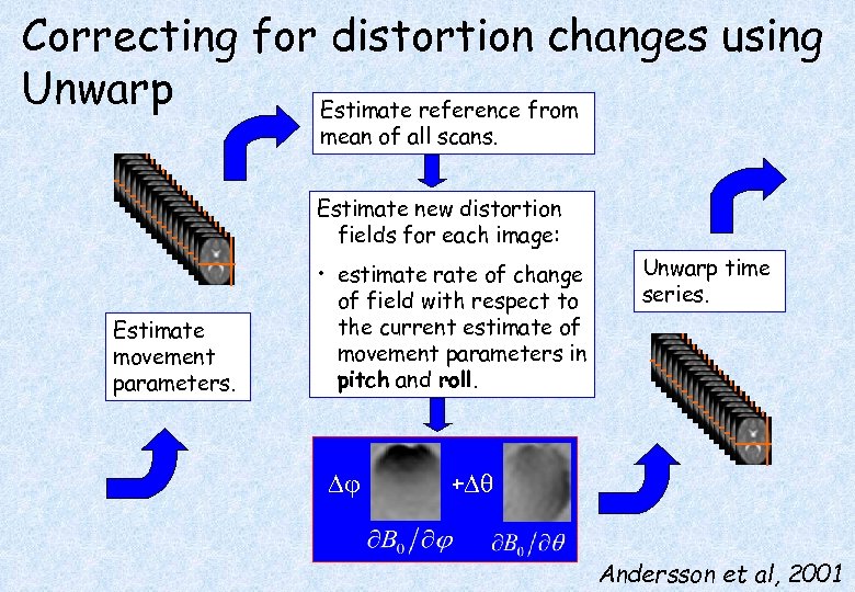
Correcting for distortion changes using Unwarp Estimate reference from mean of all scans. Estimate new distortion fields for each image: Estimate movement parameters. • estimate rate of change of field with respect to the current estimate of movement parameters in pitch and roll. Unwarp time series. + Andersson et al, 2001

Contents z. Smoothing z. Rigid registration z. Spatial normalisation y. Affine registration y. Nonlinear registration y. Regularisation

Spatial Normalisation - Reasons z. Inter-subject averaging y. Increase sensitivity with more subjects x. Fixed-effects analysis y. Extrapolate findings to the population as a whole x. Mixed-effects analysis z. Standard coordinate system ye. g. , Talairach & Tournoux space

Spatial Normalisation - Objective z. Warp the images such that functionally homologous regions from different subjects are as close together as possible y. Problems: x. No exact match between structure and function x. Different brains are organised differently x. Computational problems (local minima, not enough information in the images, computationally expensive) z. Compromise by correcting gross differences followed by smoothing of normalised images

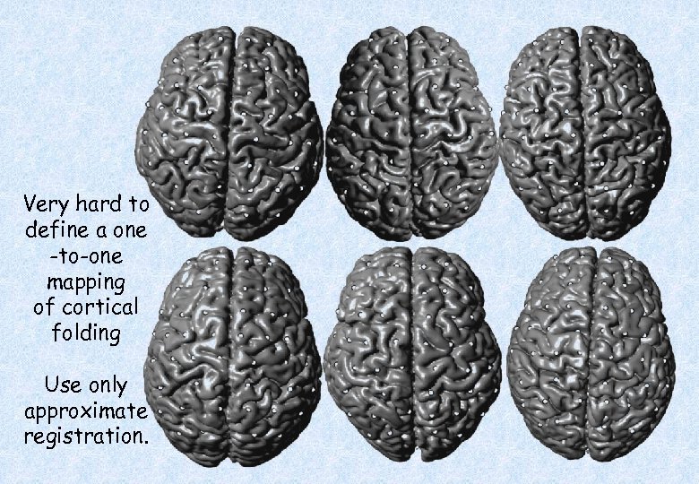
Very hard to define a one -to-one mapping of cortical folding Use only approximate registration.

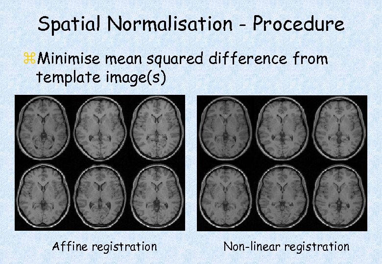
Spatial Normalisation - Procedure z. Minimise mean squared difference from template image(s) Affine registration Non-linear registration

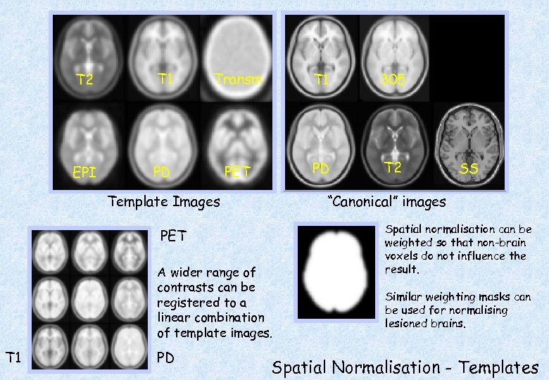
T 2 T 1 Transm T 1 305 EPI PD PET PD T 2 Template Images “Canonical” images PET A wider range of contrasts can be registered to a linear combination of template images. T 1 PD SS Spatial normalisation can be weighted so that non-brain voxels do not influence the result. Similar weighting masks can be used for normalising lesioned brains. Spatial Normalisation - Templates

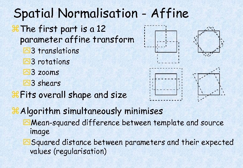
Spatial Normalisation - Affine z The first part is a 12 parameter affine transform y 3 translations y 3 rotations y 3 zooms y 3 shears z Fits overall shape and size z Algorithm simultaneously minimises y. Mean-squared difference between template and source image y. Squared distance between parameters and their expected values (regularisation)

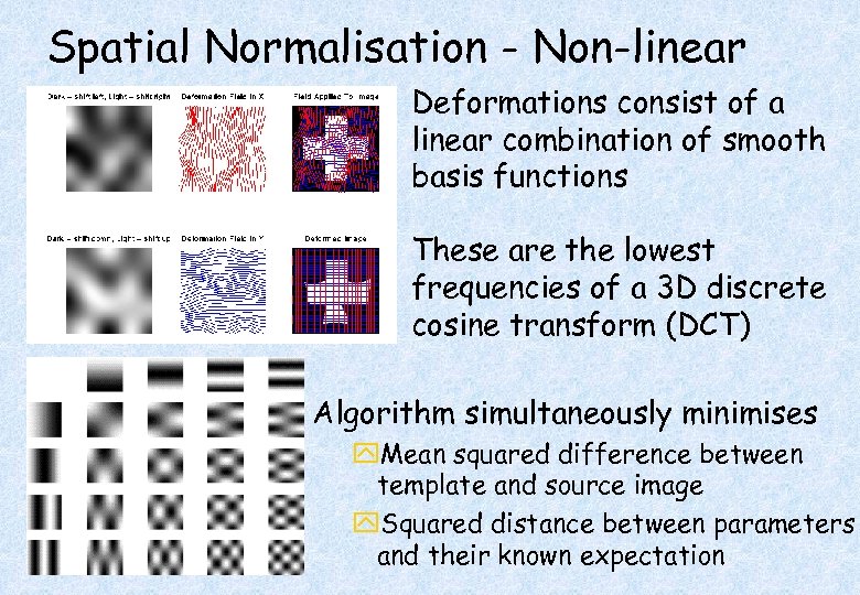
Spatial Normalisation - Non-linear Deformations consist of a linear combination of smooth basis functions These are the lowest frequencies of a 3 D discrete cosine transform (DCT) Algorithm simultaneously minimises y. Mean squared difference between template and source image y. Squared distance between parameters and their known expectation

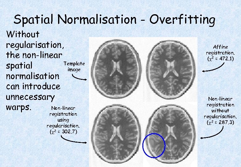
Spatial Normalisation - Overfitting Without regularisation, the non-linear Template spatial image normalisation can introduce unnecessary Non-linear warps. registration using regularisation. ( 2 = 302. 7) Affine registration. ( 2 = 472. 1) Non-linear registration without regularisation. ( 2 = 287. 3)

References Friston et al (1995): Spatial registration and normalisation of images. Human Brain Mapping 3: 165 -189 Collignon et al (1995): Automated multi-modality image registration based on information theory. IPMI’ 95 pp 263 -274 Andersson et al (2001): Modeling geometric deformations in EPI time series. Neuroimage 13: 903 -919 Thévenaz et al (2000): Interpolation revisited. IEEE Trans. Med. Imaging 19: 739 -758. Ashburner et al (1997): Incorporating prior knowledge into image registration. Neuro. Image 6: 344 -352 Ashburner et al (1999): Nonlinear spatial normalisation using basis functions. Human Brain Mapping 7: 254 -266