338bc7411e325ade55fdc1a6960e2ff6.ppt
- Количество слайдов: 108
 South Dakota School of Mines & Technology Introduction to Probability & Statistics Industrial Engineering
 South Dakota School of Mines & Technology Applications in Quality Industrial Engineering
 South Dakota School of Mines & Technology Acceptance Sampling Industrial Engineering
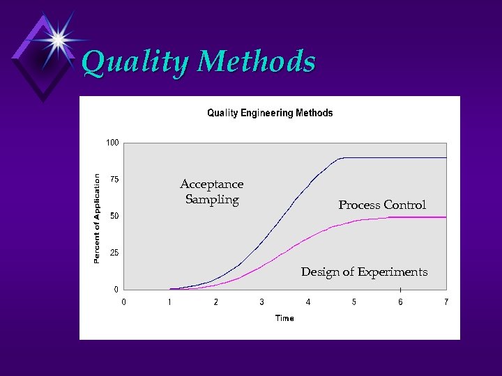 Quality Methods Acceptance Sampling Process Control Design of Experiments
 Quality Design & Process Variation Lower Spec Limit Acceptance Sampling 60 80 Upper Spec Limit 100 120 140 Statistical Process Control 60 140 Experimental Design 60 140
 Acceptance Sampling Suppose we buy parts in lot sizes of 5, 000 and we wish to inspect to ensure that the incoming quality is sufficient. Obviously, we would not like to do 100% inspection. Idea: Select a portion, n, of the lot at random and determine the number of defects in the sample. If the number of defects, d, surpasses some critical value, c, assume the entire lot is defective and ship it back.
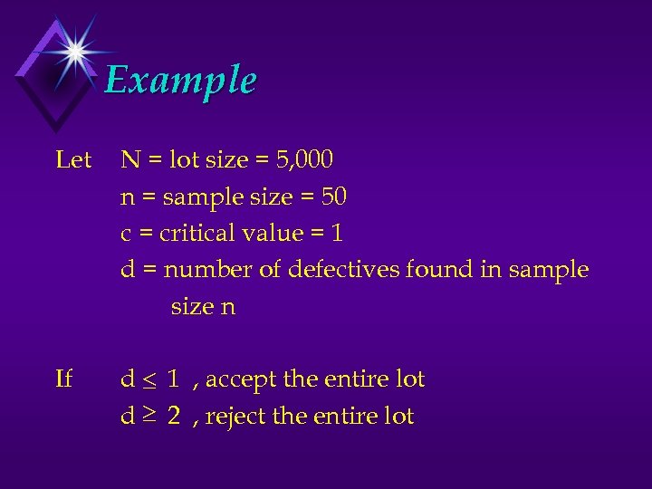 Example Let N = lot size = 5, 000 n = sample size = 50 c = critical value = 1 d = number of defectives found in sample size n If d 1 , accept the entire lot d 2 , reject the entire lot
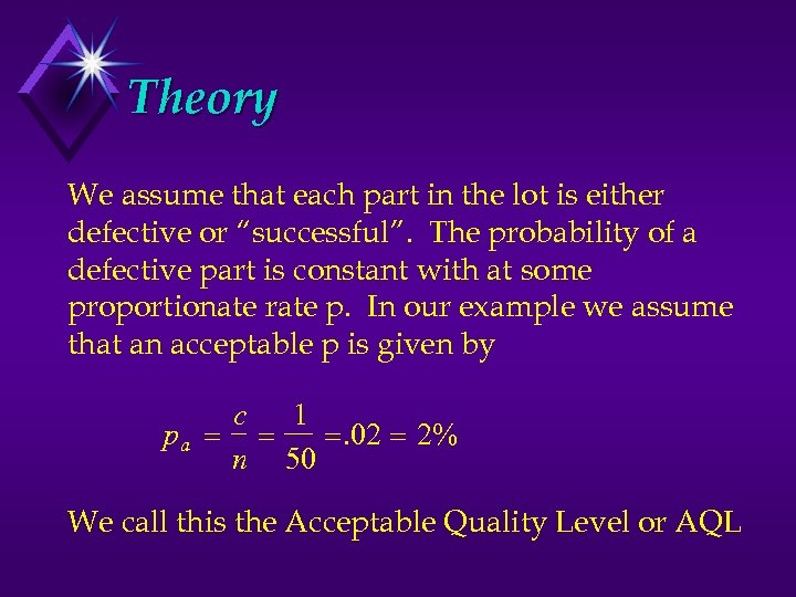 Theory We assume that each part in the lot is either defective or “successful”. The probability of a defective part is constant with at some proportionate rate p. In our example we assume that an acceptable p is given by c 1 pa . 02 2% n 50 We call this the Acceptable Quality Level or AQL
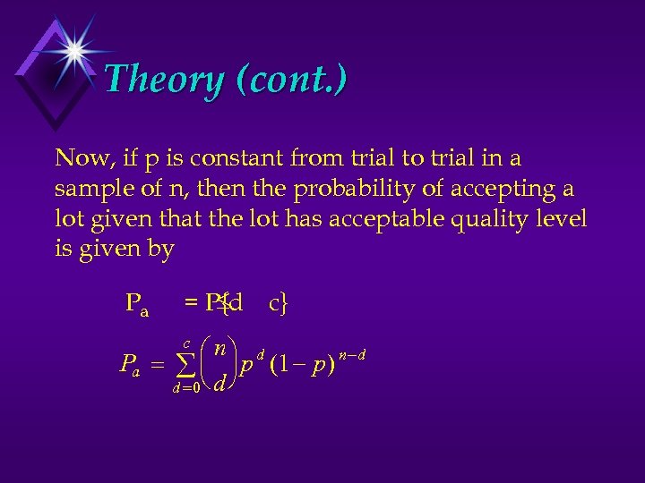 Theory (cont. ) Now, if p is constant from trial to trial in a sample of n, then the probability of accepting a lot given that the lot has acceptable quality level is given by Pa = P{d c} n p d (1 p ) n d Pa d 0 d c
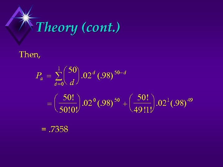 Theory (cont. ) Then, 50 . 02 d (. 98) 50 d Pa d 0 d 1 50! . 02 0 (. 98) 50 50! . 02 1 (. 98) 49 50!0! 49 !1! =. 7358
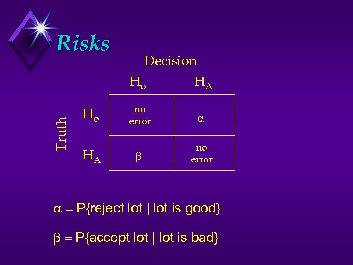 Truth Risks Ho HA Decision Ho HA no error P{reject lot | lot is good} P{accept lot | lot is bad}
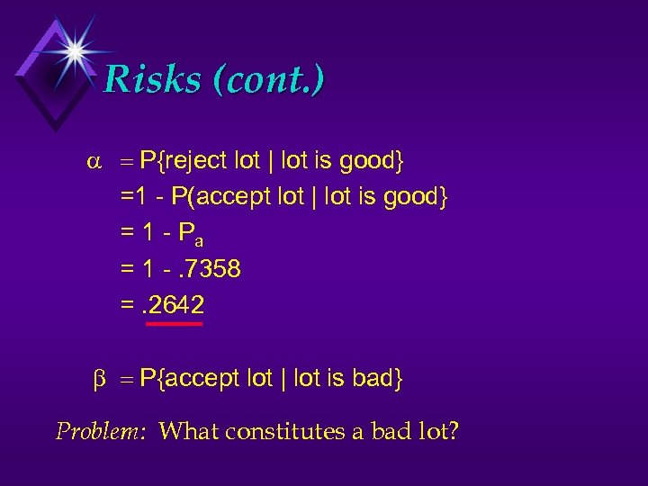 Risks (cont. ) P{reject lot | lot is good} =1 - P(accept lot | lot is good} = 1 - Pa = 1 -. 7358 =. 2642 P{accept lot | lot is bad} Problem: What constitutes a bad lot?
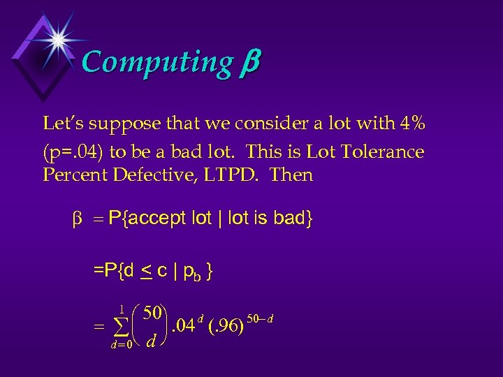 Computing Let’s suppose that we consider a lot with 4% (p=. 04) to be a bad lot. This is Lot Tolerance Percent Defective, LTPD. Then P{accept lot | lot is bad} =P{d < c | pb } 50 . 04 d (. 96) 50 d d 0 d 1
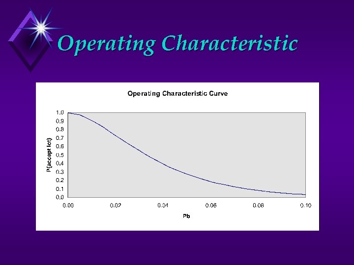
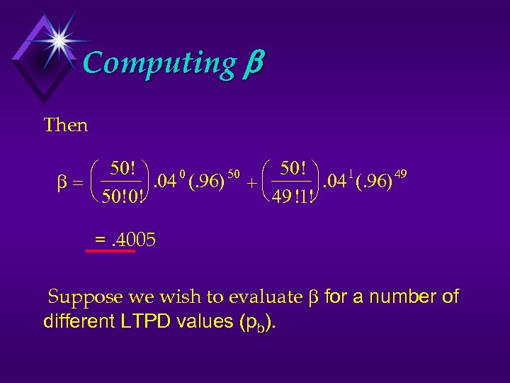 Computing Then 50! . 04 0 (. 96) 50 50! . 04 1 (. 96) 49 50!0! 49 !1! =. 4005 Suppose we wish to evaluate for a number of different LTPD values (pb).
 Operating Characteristic
 Acceptance Sampling u Uses u when testing is destructive u cost of 100% inspection is high u inspection error rate is high u cost of passing limited number of defective products is low u the process is stable
 Acceptance Sampling u Limitations u does not estimate lot quality u does not provide for quality control u risks associated with accepting bad lots and rejecting good lots u Today’s Trends u high quality u small lots FRO’s find Acceptance Sampling of little use

 South Dakota School of Mines & Technology Introductory SPC The “Magnificent 7” Industrial Engineering
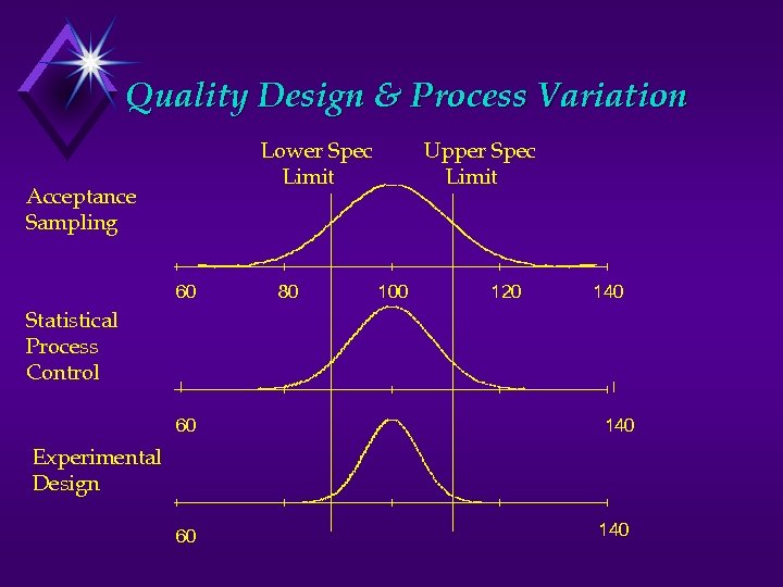 Quality Design & Process Variation Lower Spec Limit Acceptance Sampling 60 80 Upper Spec Limit 100 120 140 Statistical Process Control 60 140 Experimental Design 60 140
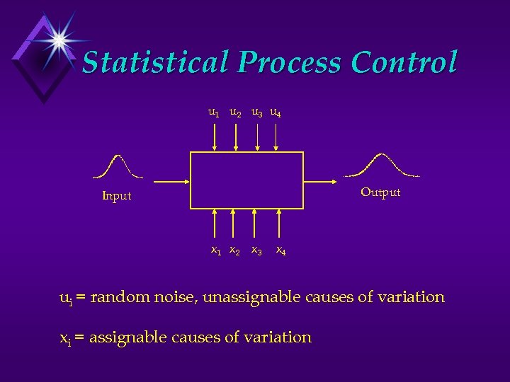 Statistical Process Control u 1 u 2 u 3 u 4 Output Input x 1 x 2 x 3 x 4 ui = random noise, unassignable causes of variation xi = assignable causes of variation
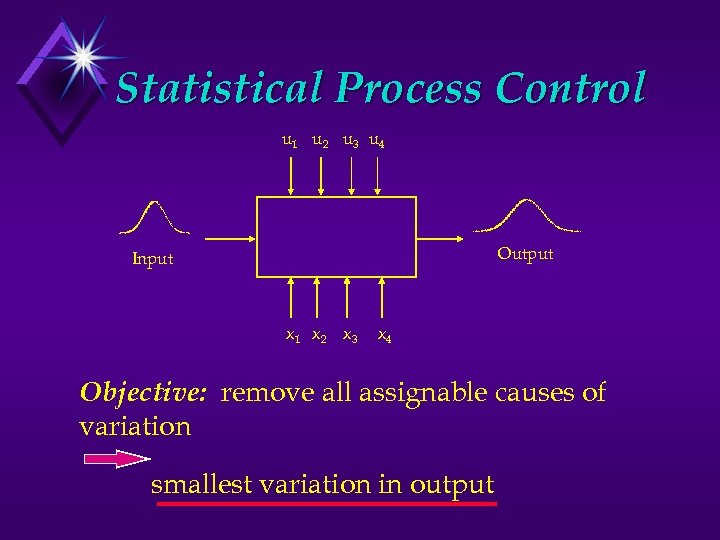 Statistical Process Control u 1 u 2 u 3 u 4 Output Input x 1 x 2 x 3 x 4 Objective: remove all assignable causes of variation smallest variation in output
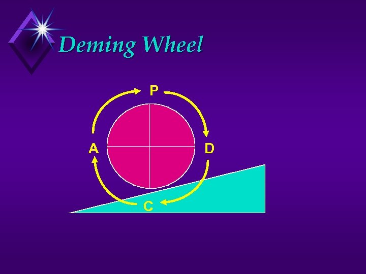 Deming Wheel P A D C
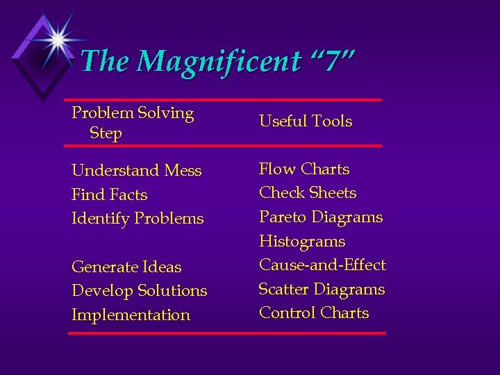 The Magnificent “ 7” Problem Solving Step Useful Tools Understand Mess Find Facts Identify Problems Flow Charts Check Sheets Pareto Diagrams Histograms Cause-and-Effect Scatter Diagrams Control Charts Generate Ideas Develop Solutions Implementation
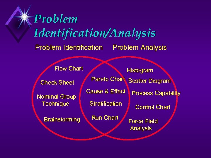 Problem Identification/Analysis Problem Identification Problem Analysis Flow Chart Histogram Check Sheet Nominal Group Technique Brainstorming Pareto Chart Scatter Diagram Cause & Effect Stratification Run Chart Process Capability Control Chart Force Field Analysis
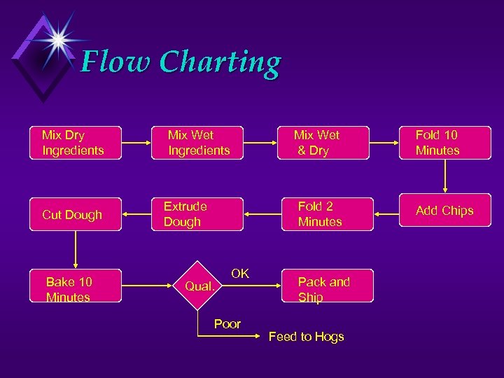 Flow Charting Mix Dry Ingredients Cut Dough Bake 10 Minutes Mix Wet Ingredients Mix Wet & Dry Extrude Dough Fold 2 Minutes Qual. OK Poor Pack and Ship Feed to Hogs Fold 10 Minutes Add Chips
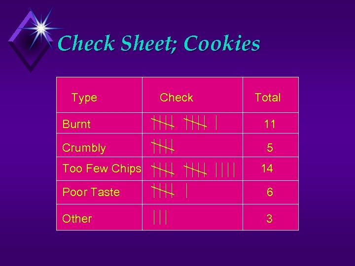 Check Sheet; Cookies Type Check Total Burnt 11 Crumbly 5 Too Few Chips 14 Poor Taste 6 Other 3
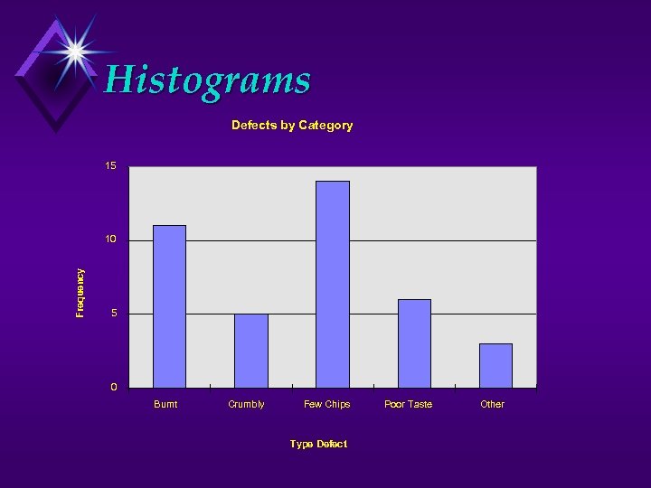 Histograms Defects by Category 15 Frequency 10 5 0 Burnt Crumbly Few Chips Type Defect Poor Taste Other
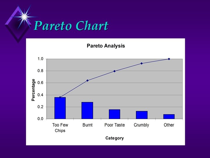 Pareto Chart
 Histogram; Class Problem u Now that we’ve decided that too few chips is our quality problem. We need to determine how many chips are in each cookie. Count your chips.
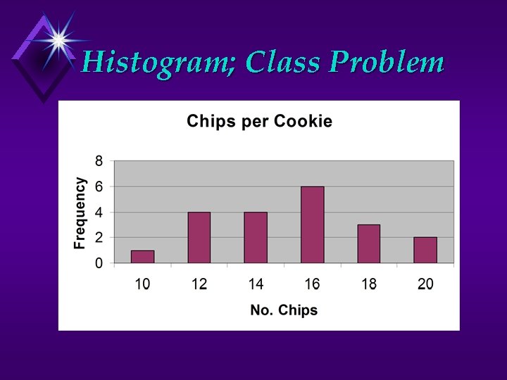 Histogram; Class Problem
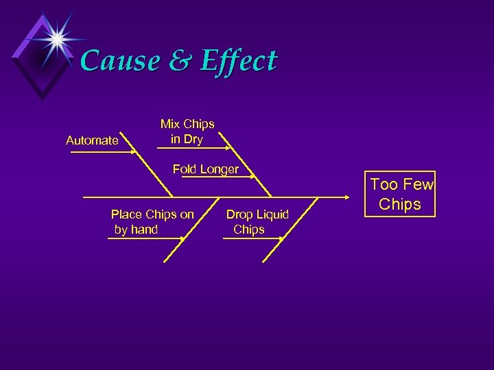 Cause & Effect Automate Mix Chips in Dry Fold Longer Place Chips on by hand Drop Liquid Chips Too Few Chips
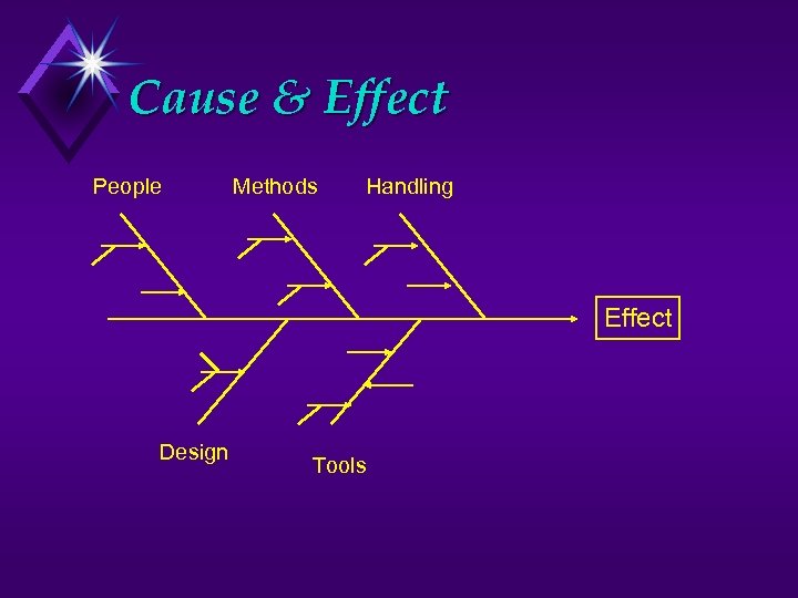 Cause & Effect People Methods Handling Effect Design Tools
 Idea; Cookies As a first step, let’s try Increasing Folding Time
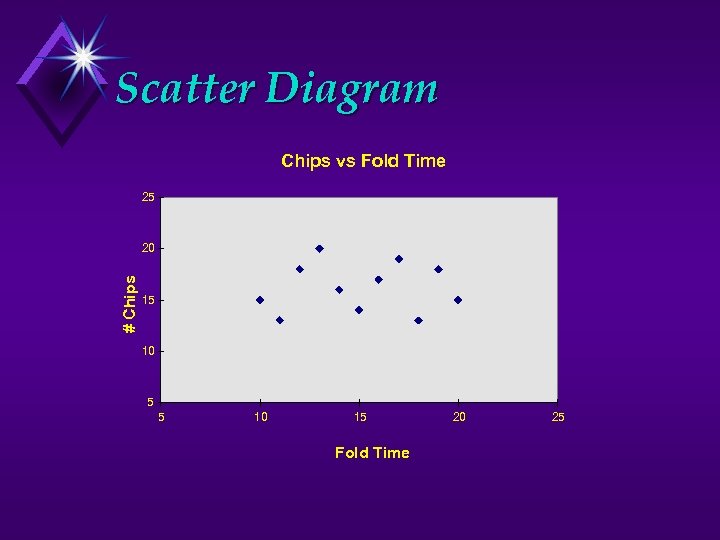 Scatter Diagram Chips vs Fold Time 25 # Chips 20 15 10 5 5 10 15 Fold Time 20 25
 New Idea; Cookies Try Mixing Chips in With Dry Ingredients
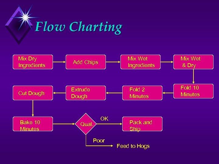 Flow Charting Mix Dry Ingredients Cut Dough Bake 10 Minutes Mix Wet Ingredients Add Chips Extrude Dough Fold 2 Minutes Qual. OK Poor Pack and Ship Feed to Hogs Mix Wet & Dry Fold 10 Minutes
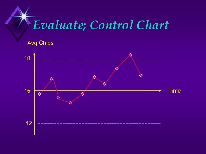 Evaluate; Control Chart Avg Chips 18 15 12 Time

 South Dakota School of Mines & Technology Control Charts Industrial Engineering
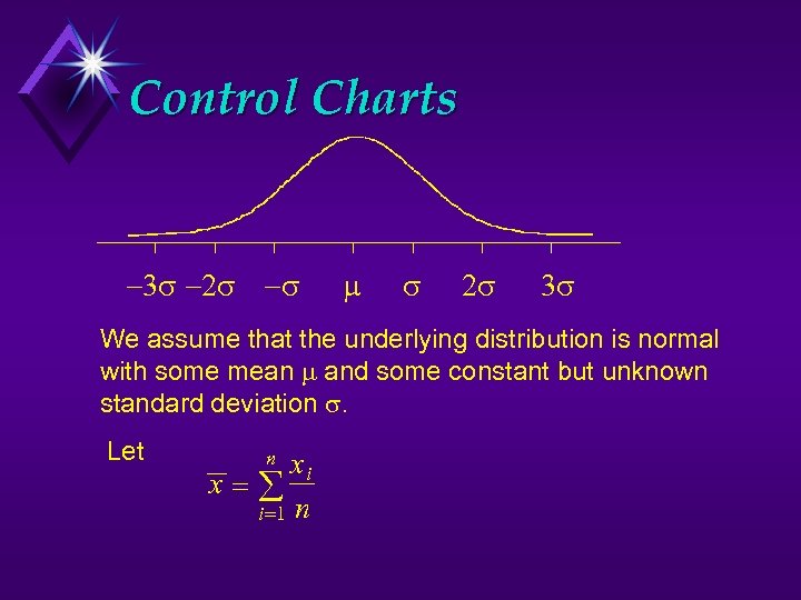 Control Charts We assume that the underlying distribution is normal with some mean and some constant but unknown standard deviation . Let xi x i 1 n n
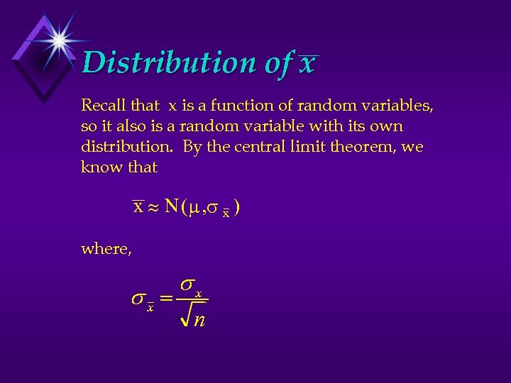 Distribution of x Recall that x is a function of random variables, so it also is a random variable with its own distribution. By the central limit theorem, we know that x N ( , x ) where, x x n
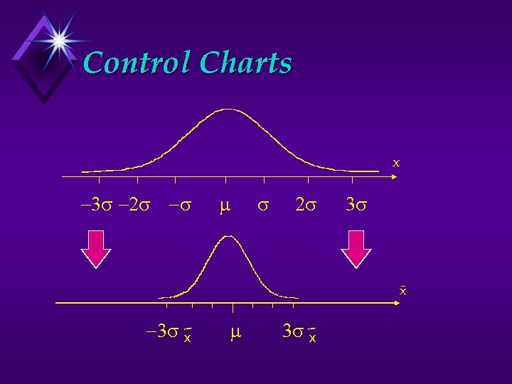 Control Charts x x x x
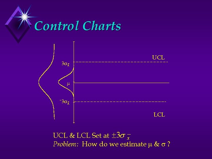 Control Charts x UCL x LCL UCL & LCL Set at 3 x Problem: How do we estimate & ?
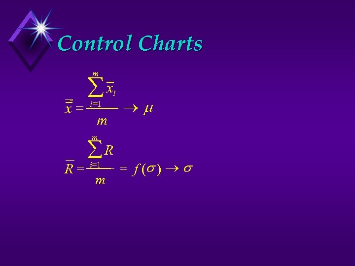 Control Charts m x x i 1 i m ® m R R i 1 m f ( ) ®
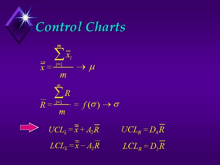 Control Charts m x x i 1 i m ® m R R i 1 m f ( ) ® UCLx x A 2 R UCLR D 4 R LCLx x A 2 R LCLR D 3 R
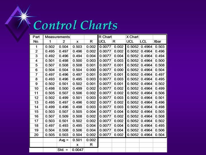
 Example u Suppose specialized o-rings are to be manufactured at. 5 inches. Too big and they won’t provide the necessary seal. Too little and they won’t fit on the shaft. Twenty samples of 2 rings each are taken. Results follow.
 Control Charts
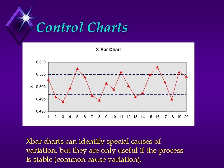 Control Charts Xbar charts can identify special causes of variation, but they are only useful if the process is stable (common cause variation).
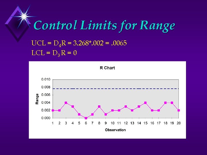 Control Limits for Range UCL = D 4 R = 3. 268*. 002 =. 0065 LCL = D 3 R = 0
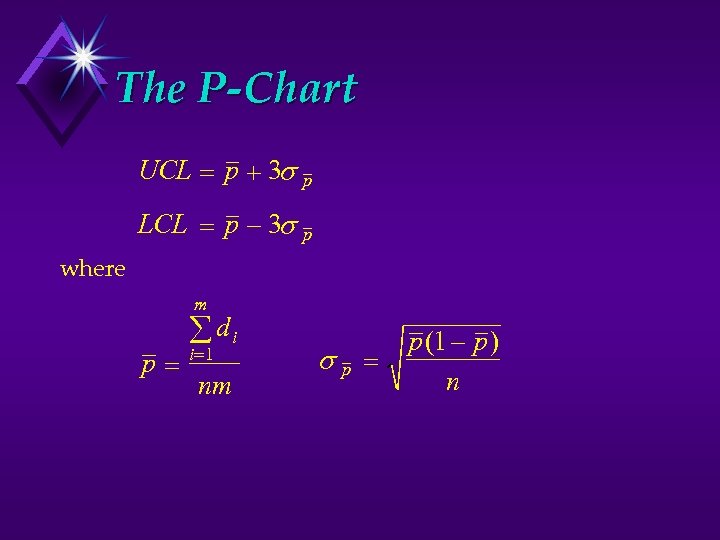 The P-Chart UCL p 3 p LCL p 3 p where m p di i 1 nm p p (1 p ) n
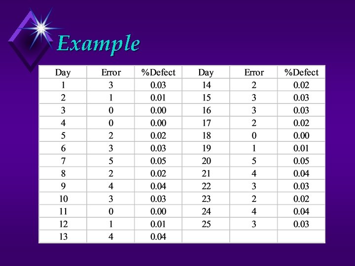
 Example; P-Chart u Operators of a sorting machine must read the zip code on a letter and diver the letter to the proper carrier route. Over one month’s time, 25 samples of 100 letters were chosen, and the number of errors was recorded. Error counts for each of the 25 days follows.
 Example
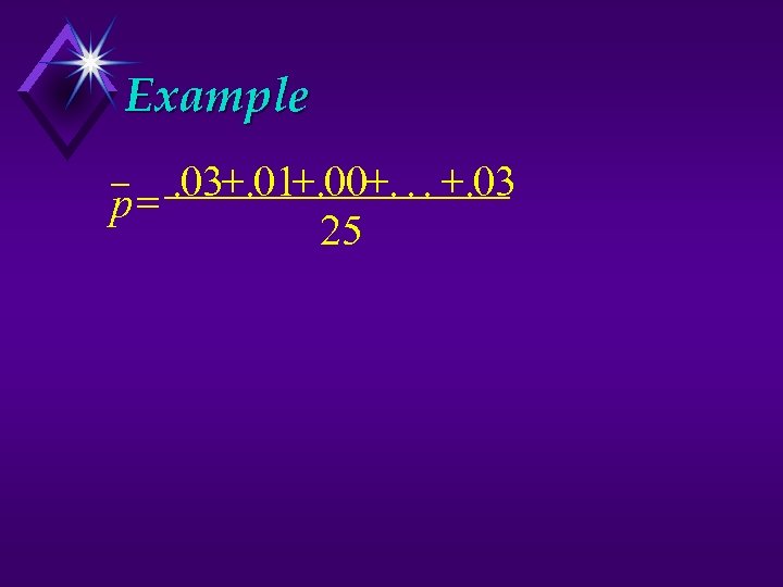 Example. 03. 01. 00. . 03 p 25
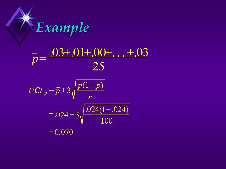 Example. 03. 01. 00. . 03 p 25 p (1 p ) UCL p p 3 n. 024(1 . 024) . 024 3 100 0. 070
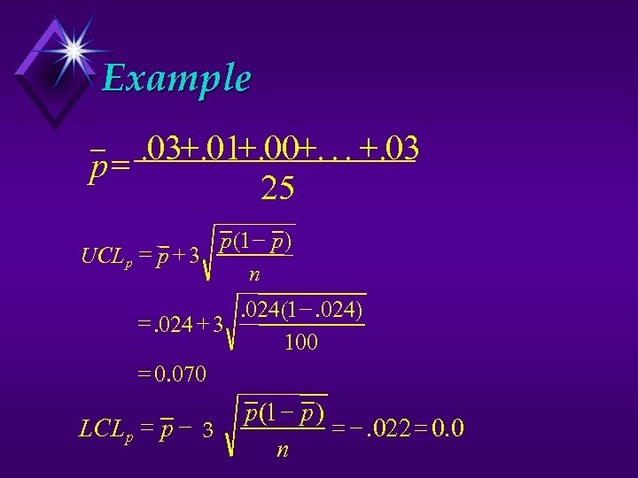 Example. 03. 01. 00. . 03 p 25 p (1 p ) UCL p p 3 n. 024(1 . 024) . 024 3 100 0. 070 LCL p p 3 p (1 p ) . 022 0. 0 n
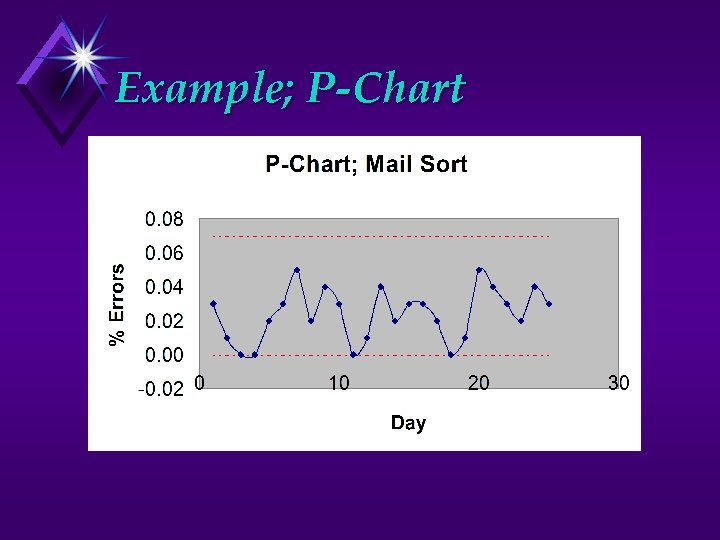 Example; P-Chart

 South Dakota School of Mines & Technology Process Capability Industrial Engineering
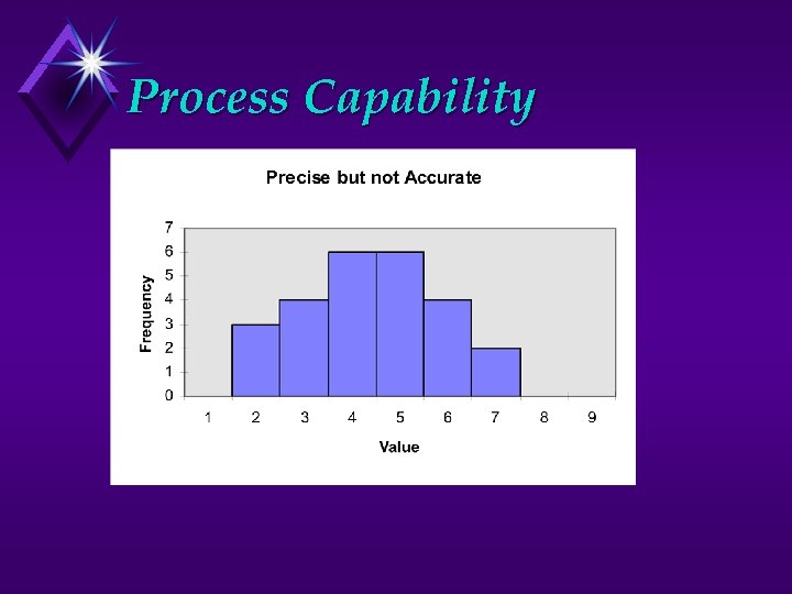 Process Capability
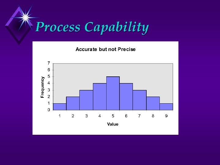 Process Capability
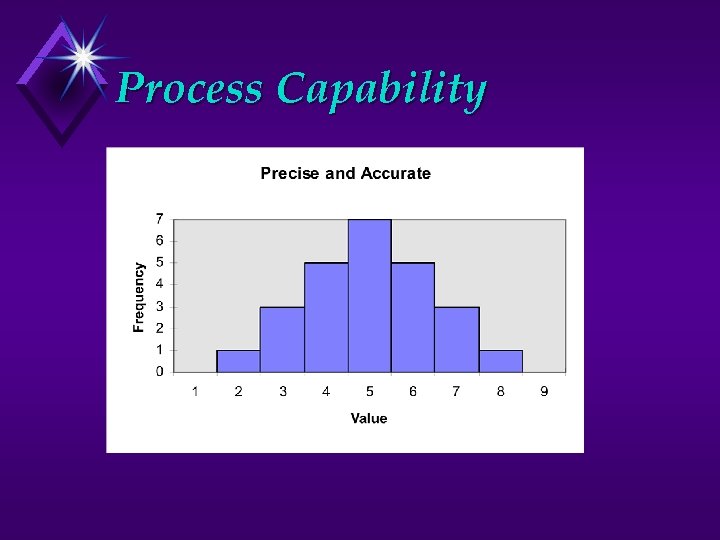 Process Capability
 Process Capability LSL USL x x USL LSL Cp 6 x
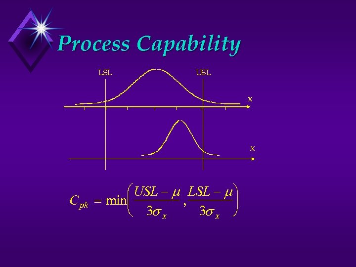 Process Capability LSL USL x x C pk USL LSL , min 3 x
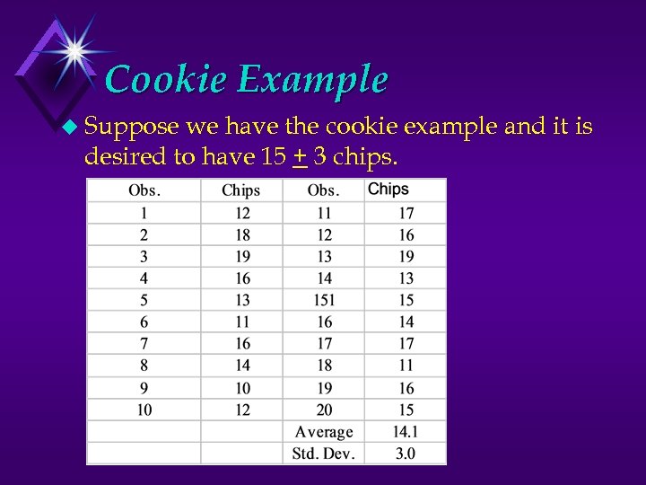 Cookie Example u Suppose we have the cookie example and it is desired to have 15 + 3 chips.
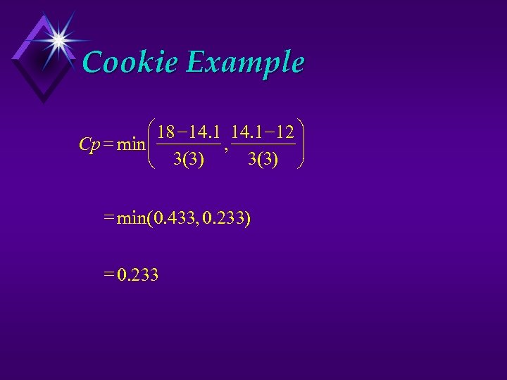 Cookie Example 18 14. 1 12 Cp min , 3(3) min(0. 433, 0. 233) 0. 233

 South Dakota School of Mines & Technology Funnel Experiment Industrial Engineering
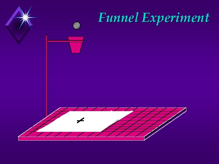
 Funnel Experiment u The Funnel Experiment is a famous experiment first developed by Dr. Deming. It was designed to show primarily two things: 1. All processes have statistical variation 2. Improving processes to reduce variation is infinitely better than trying to control process variation
 Funnel Experiment
 Funnel Experiment Rule 1: Do nothing Rule 2: Move the funnel in an equal but opposite direction Rule 3: Move the funnel in an equal but opposite direction from (0, 0) Rule 4: Move the funnel to the last position where the last hit.
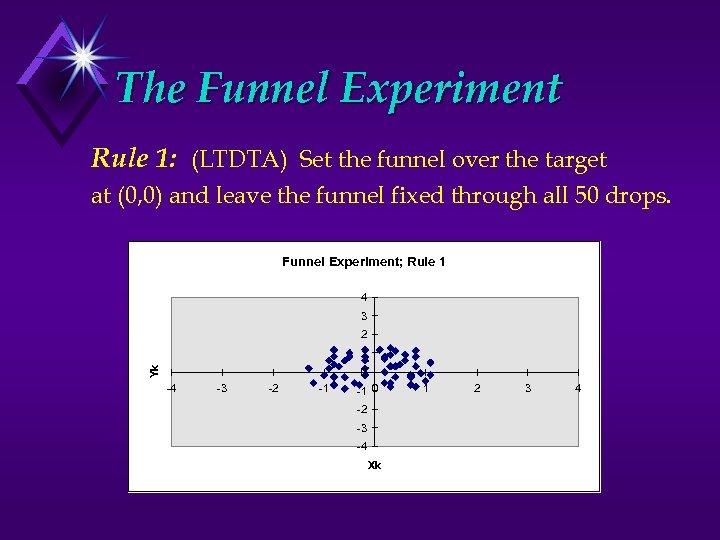 The Funnel Experiment Rule 1: (LTDTA) Set the funnel over the target at (0, 0) and leave the funnel fixed through all 50 drops. Funnel Experiment; Rule 1 4 3 2 Yk 1 0 -4 -3 -2 -1 -1 0 -2 -3 -4 Xk 1 2 3 4
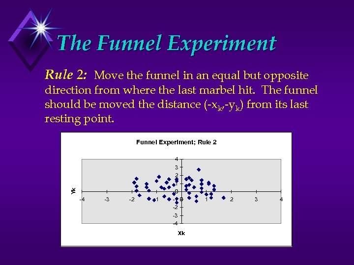 The Funnel Experiment Rule 2: Move the funnel in an equal but opposite direction from where the last marbel hit. The funnel should be moved the distance (-xk, -yk) from its last resting point. Yk Funnel Experiment; Rule 2 -4 -3 -2 -1 4 3 2 1 0 -2 -3 -4 Xk 1 2 3 4
 The Funnel Experiment Rule 2: Move the funnel in an equal but opposite direction from where the last marbel hit. The funnel should be moved the distance (-xk, -yk) from its last resting point. Machine/Process adjustment rules using control chart limits. Automatic compensating machinery
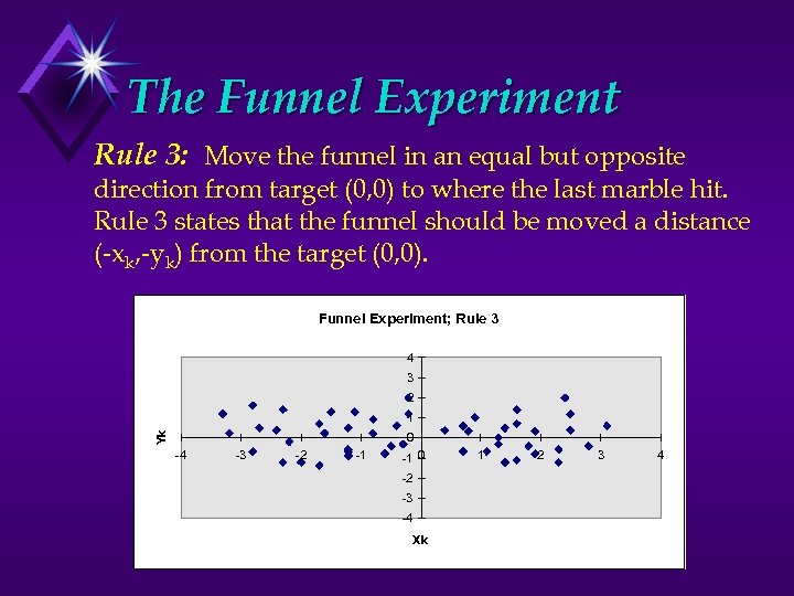 The Funnel Experiment Rule 3: Move the funnel in an equal but opposite direction from target (0, 0) to where the last marble hit. Rule 3 states that the funnel should be moved a distance (-xk, -yk) from the target (0, 0). Funnel Experiment; Rule 3 4 3 2 Yk 1 0 -4 -3 -2 -1 -1 0 -2 -3 -4 Xk 1 2 3 4
 The Funnel Experiment Rule 3: Move the funnel in an equal but opposite direction from target (0, 0) to where the last marble hit. Rule 3 states that the funnel should be moved a distance (-xk, -yk) from the target (0, 0). Management by Objectives Committees
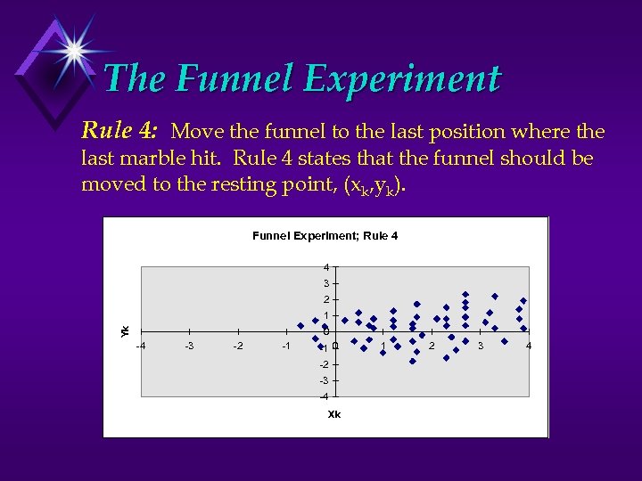 The Funnel Experiment Rule 4: Move the funnel to the last position where the last marble hit. Rule 4 states that the funnel should be moved to the resting point, (xk, yk). Funnel Experiment; Rule 4 4 3 2 Yk 1 0 -4 -3 -2 -1 -1 0 -2 -3 -4 Xk 1 2 3 4
 The Funnel Experiment Rule 4: Move the funnel to the last position where the last marble hit. Rule 4 states that the funnel should be moved to the resting point, (xk, yk). Operator matches color from batch to batch without reference to original swatch. Operator attempts to make every piece like the last one. On the job training.
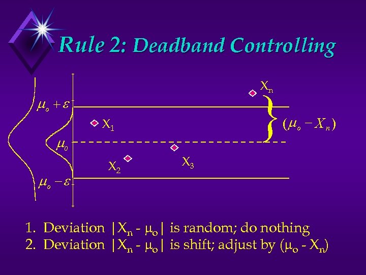 Rule 2: Deadband Controlling Xn } o e o o e X 1 X 2 ( o X n ) X 3 1. Deviation |Xn - o| is random; do nothing 2. Deviation |Xn - o| is shift; adjust by ( o - Xn)
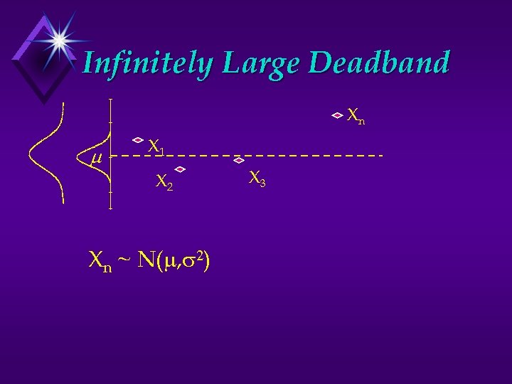 Infinitely Large Deadband Xn X 1 X 2 Xn ~ N( , ) X 3
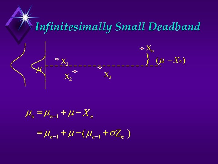 Infinitesimally Small Deadband Xn } X 1 X 2 X 3 n n 1 X n n 1 ( n 1 Zn ) ( X n )
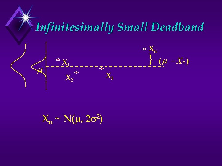 Infinitesimally Small Deadband Xn } X 1 X 2 Xn ~ N( , 2 2) X 3 ( X n )
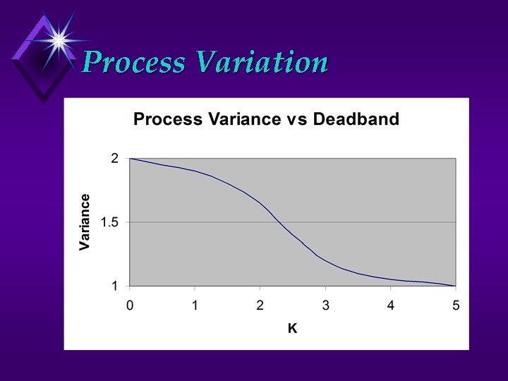 Process Variation

 South Dakota School of Mines & Technology Loss Functions Industrial Engineering
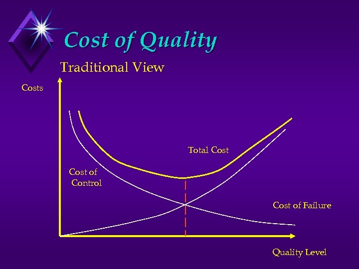 Cost of Quality Traditional View Costs Total Cost of Control Cost of Failure Quality Level
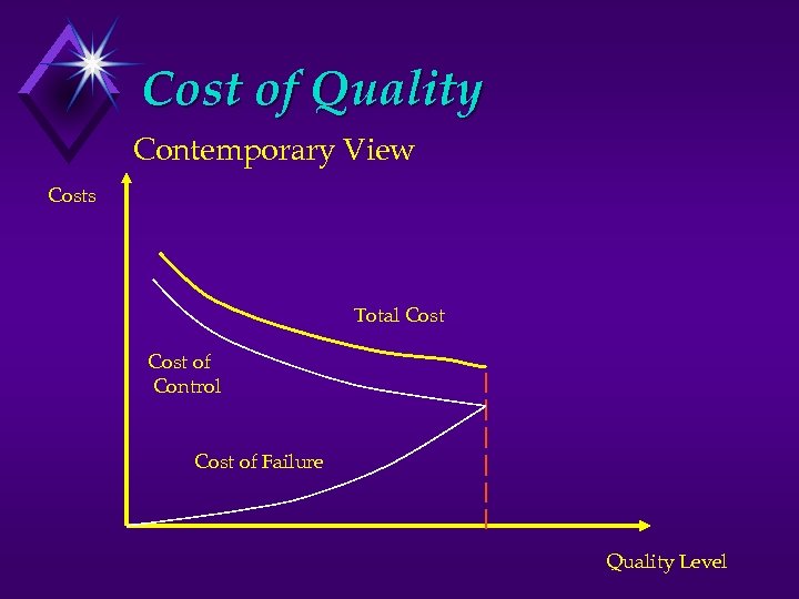 Cost of Quality Contemporary View Costs Total Cost of Control Cost of Failure Quality Level
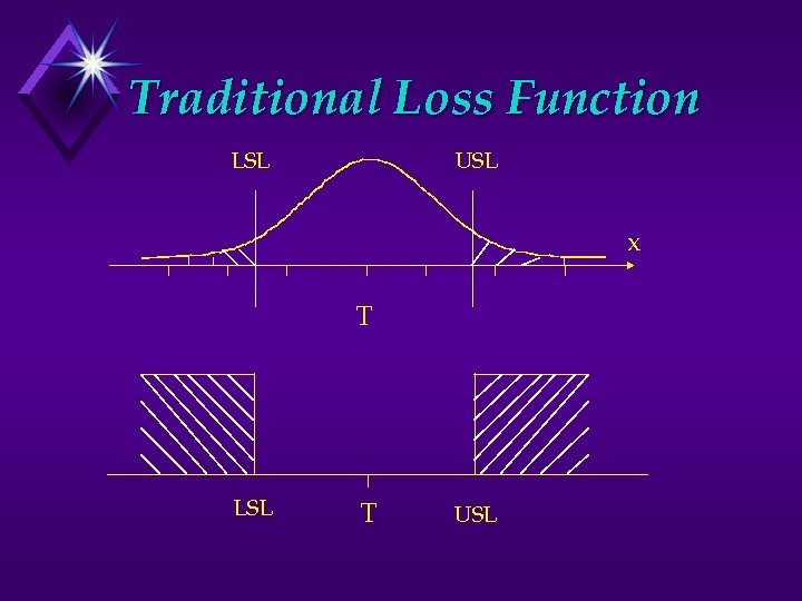 Traditional Loss Function LSL USL x T LSL T USL
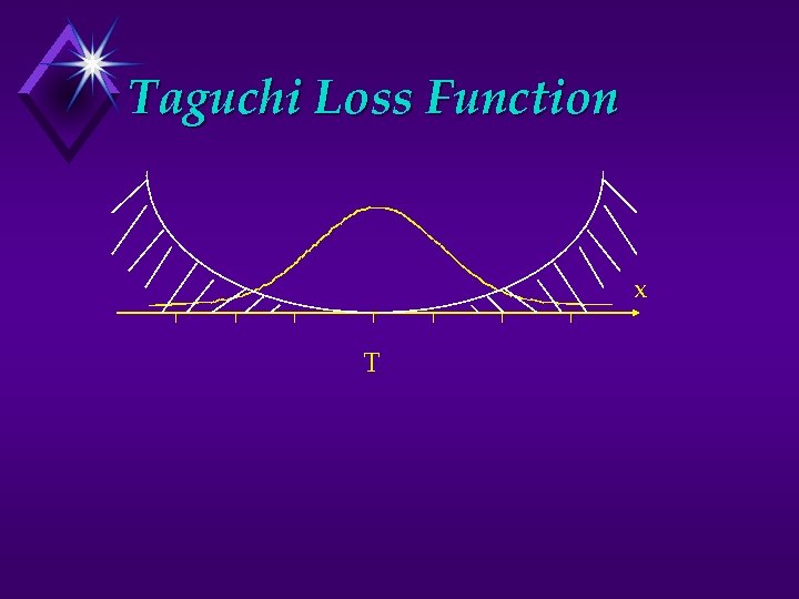 Taguchi Loss Function x T
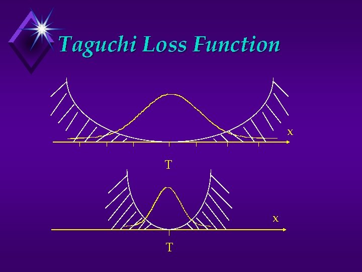 Taguchi Loss Function x T
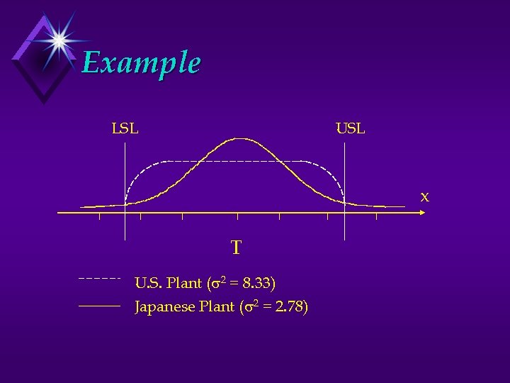
 Example (Sony, 1979) Comparing cost of two Sony television plants in Japan and San Diego. All units in San Diego fell within specifications. Japanese plant had units outside of specifications. Loss per unit (Japan) = $0. 44 Loss per unit (San Diego) = $1. 33 How can this be? Sullivan, “Reducing Variability: A New Approach to Quality, ” Quality Progress, 17, no. 7, 15 -21, 1984.
 Example LSL USL x T U. S. Plant ( 2 = 8. 33) Japanese Plant ( 2 = 2. 78)
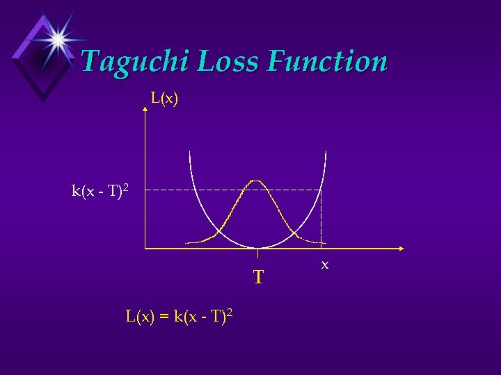 Taguchi Loss Function L(x) k(x - T)2 T L(x) = k(x - T)2 x
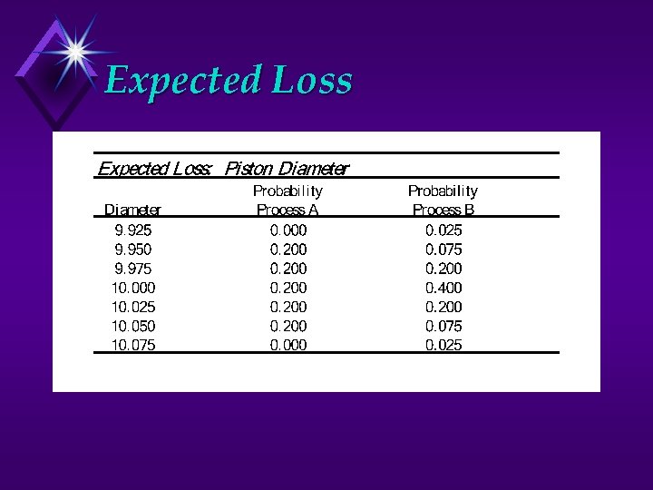
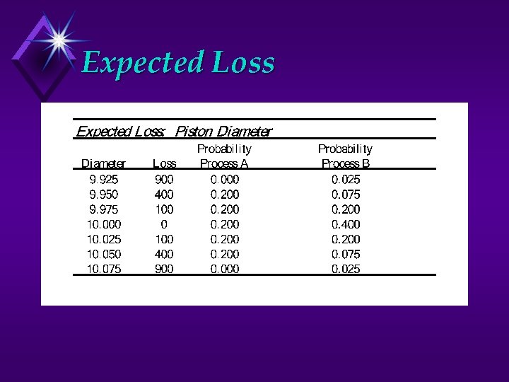
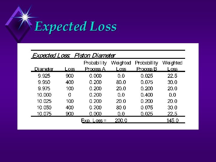
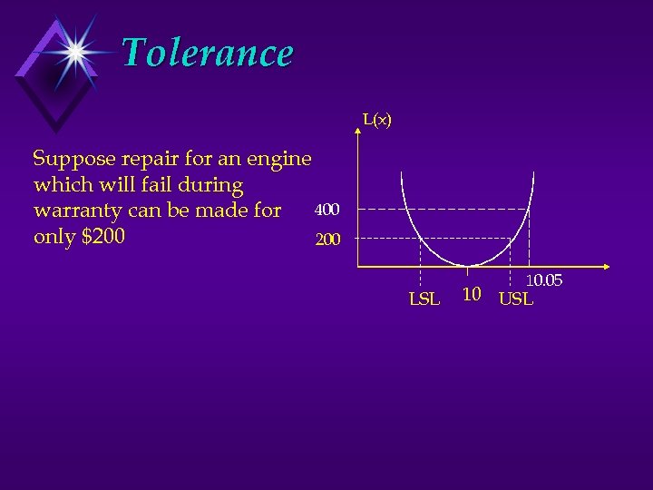
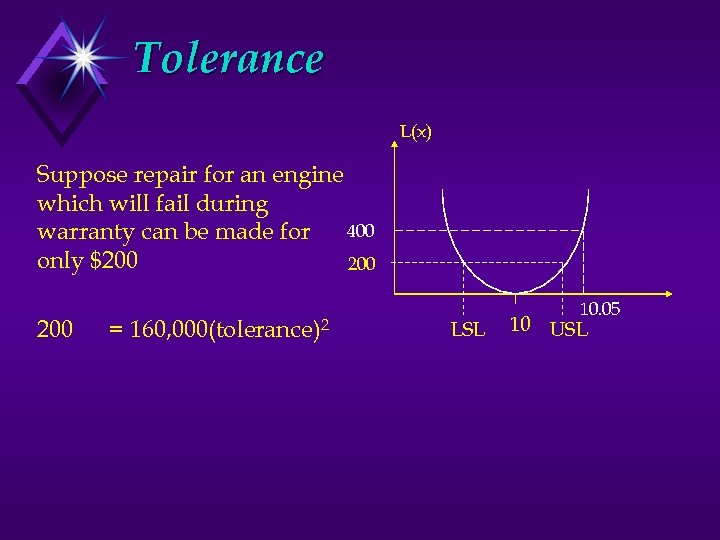
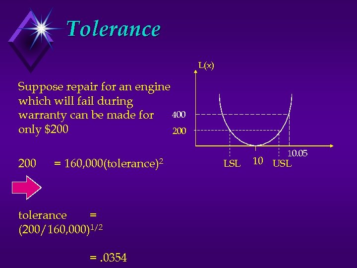
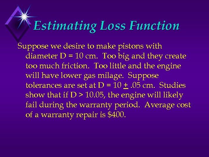 Estimating Loss Function Suppose we desire to make pistons with diameter D = 10 cm. Too big and they create too much friction. Too little and the engine will have lower gas milage. Suppose tolerances are set at D = 10 +. 05 cm. Studies show that if D > 10. 05, the engine will likely fail during the warranty period. Average cost of a warranty repair is $400.
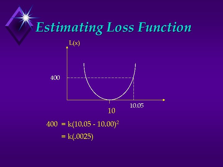 Estimating Loss Function L(x) 400 10 400 = k(10. 05 - 10. 00)2 = k(. 0025) 10. 05
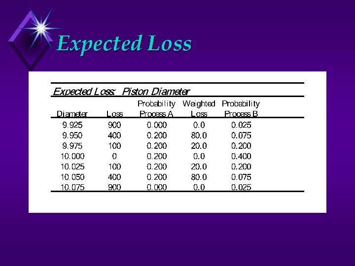
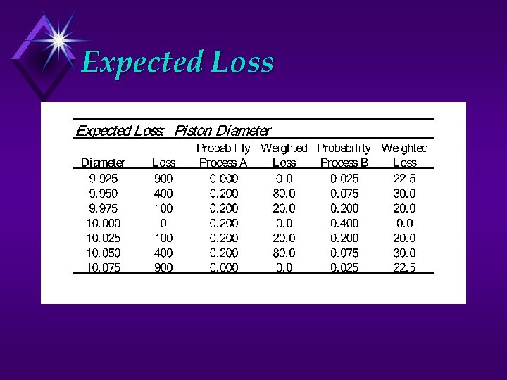
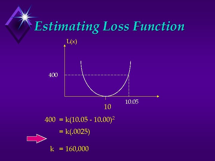 Estimating Loss Function L(x) 400 10 400 = k(10. 05 - 10. 00)2 = k(. 0025) k = 160, 000 10. 05
 Expected Loss
 Expected Loss
 Expected Loss
 Expected Loss
 Expected Loss
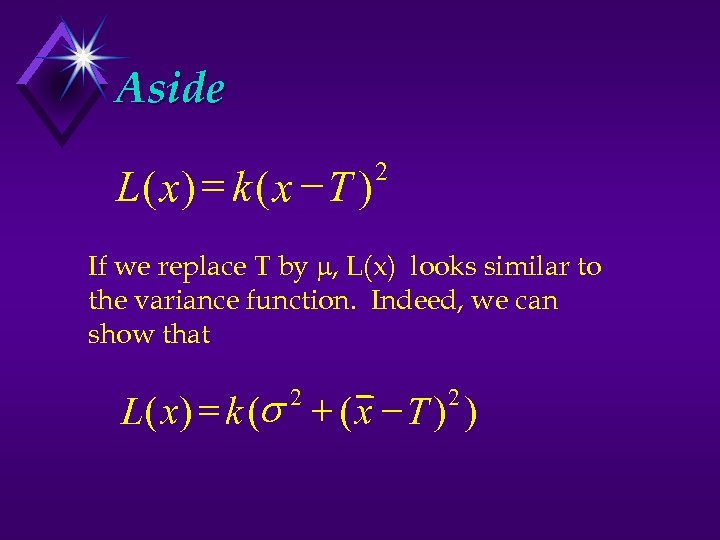 Aside L( x) k ( x T ) 2 If we replace T by , L(x) looks similar to the variance function. Indeed, we can show that L( x) k ( ( x T ) ) 2 2
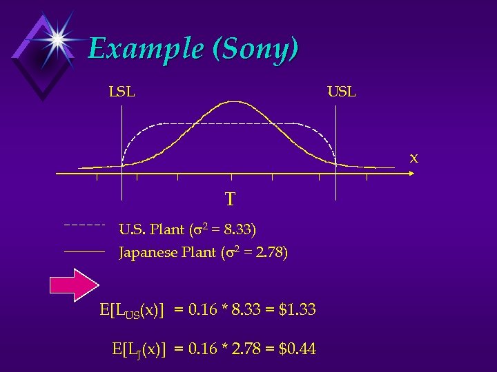 Example (Sony) LSL USL x T U. S. Plant ( 2 = 8. 33) Japanese Plant ( 2 = 2. 78) E[LUS(x)] = 0. 16 * 8. 33 = $1. 33 E[LJ(x)] = 0. 16 * 2. 78 = $0. 44
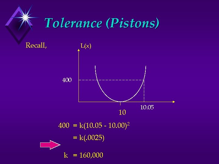 Tolerance (Pistons) Recall, L(x) 400 10 400 = k(10. 05 - 10. 00)2 = k(. 0025) k = 160, 000 10. 05
 Tolerance L(x) Suppose repair for an engine which will fail during 400 warranty can be made for only $200 LSL 10. 05 10 USL
 Tolerance L(x) Suppose repair for an engine which will fail during 400 warranty can be made for only $200 200 = 160, 000(tolerance)2 LSL 10. 05 10 USL
 Tolerance L(x) Suppose repair for an engine which will fail during 400 warranty can be made for only $200 200 = 160, 000(tolerance)2 tolerance = (200/160, 000)1/2 =. 0354 LSL 10. 05 10 USL


