Some further problems with regression models Regression analysis

Some further problems with regression models Regression analysis has two fundamental tasks: 1. Estimation: computing from sample data reliable estimates of the numerical values of the regression coefficients βj (j = 0, 1, …, k), and hence of the population regression function. 2. Inference: using sample estimates of the regression coefficients βj (j = 0, 1, …, k) to test hypotheses about the population values of the unknown regression coefficients -- i. e. , to infer from sample estimates the true population values of the regression coefficients within specified margins of statistical error.

CONFIDENCE INTERVALS FOR PARAMETERS Let the population regression model be Let b 0, b 1 , . . , b. K be the least squares estimates of the population parameters and sb 0, sb 1, . . . , sb. K be the estimated standard deviations of the least squares estimators (square roots from the diagonal items of variance-covariance matrix). Then if the standard regression assumptions hold and if the error terms i are normally distributed, the random variables corresponding to are distributed as Student’s t with (n – k – 1) degrees of freedom.

CONFIDENCE INTERVALS FOR PARAMETERS If the regression errors i , are normally distributed and the standard regression assumptions hold, the 100(1 - )% confidence intervals for the partial regression coefficients j, are given by and the random variable t(n – k - 1) follows a Student’s t distribution with (n – k - 1) degrees of freedom.

STANDARD ERROR FOR REGRESSION PARAMETERS Y-weekly salary ($) X 1 –length of employment (months) X 2 -age (years) Se 2

STANDARD ERROR FOR REGRESSION PARAMETERS variance-covariance matrix β 0 differs from b 0 for 57 units. β 1 differs from b 1 0, 15 units. β 2 differs from b 2 for 1, 77 units.

CONFIDENCE INTERVALS FOR PARAMETERS t-Student statistic for the level of significance 0, 05 and df=13 is 2, 160 Confidence interval for β 0 Interval with the lower limit 338, 3508 $ and the upper limit 585, 3495$ covers the unknown value of parameter β 0 (for population) with 95% probability.

CONFIDENCE INTERVALS FOR PARAMETERS t-Student statistic for the level of significance 0, 05 and df=13 is 2, 160 Confidence interval for β 1 Interval with the lower limit 0, 3526 $ and the upper limit 0, 9898$ covers the unknown value of parameter β 1 (for population) with 95% probability.

CONFIDENCE INTERVALS FOR PARAMETERS t-Student statistic for the level of significance 0, 05 and df=13 is 2, 160 Confidence interval for β 2 Interval with the lower limit – 5, 2124$ and the upper limit 2, 4456$ covers the unknown value of parameter β 2 (for population) with 95% probability.

TESTING ALL THE PARAMETERS OF A MODEL Consider the multiple regression model To test the null hypothesis against the alternative hypothesis at a significance level we can use the decision rule where F , k, n–k– 1 is the critical value of F the computed F k, n–k– 1 follows an F distribution with numerator degrees of freedom k and denominator degrees of freedom (n–k– 1)

TESTING ALL THE PARAMETERS OF A MODEL F-value computed from the sample F-value from F tables F , k, n–k– 1 = F 0, 05, 2, 13= 3, 81 F comp > Fα, k, n-k-1 We reject the null hypothesis. 28, 448 >3, 81 At least one parameter is statistically significant.

TESTING SINGLE PARAMETER OF A MODEL If the regression errors are normally distributed and the standard least squares assumptions hold, the following tests have significance level : To test either null hypothesis against the alternative the decision rule is

TESTING PARAMETERS OF A MODEL INDIVIDUALLY TESTING SINGLE PARAMETER OF A MODEL To test either null hypothesis against the two-sided alternative the decision rule is

TESTING PARAMETERS OF A MODEL INDIVIDUALLY TESTING SINGLE PARAMETER OF A MODEL Y-weekly salary ($) X 1 –length of employment (months) X 2 -age (years) The null hypothesis can better be stated as: independent variable Xj does not contribute to the prediction of Y, given that other independent variables already have been included in the model The alternative hypothesis can better be stated as: independent variable Xj does contribute to the prediction of Y, given that other independent variables already have been included in the model

TESTING PARAMETERS OF A MODEL INDIVIDUALLY TESTING SINGLE PARAMETER OF A MODEL Y-weekly salary ($) X 1 –length of employment (months) X 2 -age (years) The length of employment (X 1) does not contribute to the prediction of weekly salary (Y), given that the age (X 2) already have been included in the model. The length of employment (X 1) does contribute to the prediction of weekly salary (Y), given that the age (X 2) already have been included in the model. t-value computed from the sample t-value from t-Student tables is 2, 16 We reject the null hypothesis. The length of employment (X 1) does contribute to the prediction of weekly salary (Y), given that the age (X 2) already have been included in the model.

TESTING PARAMETERS OF A MODEL INDIVIDUALLY TESTING SINGLE PARAMETER OF A MODEL Y-weekly salary ($) X 1 –length of employment (months) X 2 -age (years) The age (X 2) does not contribute to the prediction of weekly salary (Y), given that the length of employment (X 1) already have been included in the model. The age (X 2) does contribute to the prediction of weekly salary (Y), given that the length of employment (X 1) already have been included in the model. t-value computed from the sample t-value from t-Student tables is 2, 16 We don’t reject the null hypothesis. The age (X 2) does not contribute to the prediction of weekly salary (Y), given that the length of employment (X 1) already have been included in the model.

LINEARITY is essential for calculation of multivariate statistics due to the basis upon the general linear model, and the assumption of multivariate normality which implies that there is linearity between all pairs of variables, with significance tests based upon that assumption. Nonlinearity may be diagnosed from bivariate scatterplots between pairs of variables or from a residual plot, with predicted values of the dependent variable versus the residuals. Residual plots may demonstrate: failure of normality, nonlinearity, and heteroscedasticity. Linearity between two variables may be assessed through observation of bivariate scatterplots. When both variables are normally distributed and linearly related, the scatterplot is oval shaped, if one of the variables is nonnormal then the scatterplot is not oval.

LINEARITY Linearity is the assumption that there is a straight line relationship between variables. Expected distribution of residuals for a linear model with normal distribution of residuals (errors).

LINEARITY Examples of non-linear distributions:

LINEARITY The positive residuals should be named with “a”, the negative – “b”. We should count the number of positive (n 1) and negative (n 2) residuals. The run is a group of residuals of the same sign (“a” or “b”). We need number of runs for our sample. This is called S. From the runs test tables we need S 1 and S 2 for the level of significance and n 1 and n 2 degrees of freedom. Decision rule: Reject H 0 if S=<S 1 or S>=S 2. The form of model (linear form) is not proper Don’t reject H 0 if S 1<S<S 2. The form of model is proper

LINEARITY

NORMALITY The underlying assumption of most multivariate analysis and statistical tests is the assumptions of multivariate normality. Multivariate normality is the assumption that all variables and all combinations of the variables are normally distributed. When the assumption is met the residuals are normally distributed and independent, the differences between predicted and obtained scores (the errors) are symmetrically distributed around a mean of zero and there is no pattern to the errors. Screening for normality may be undertaken in either statistical or graphical methods.

NORMALITY

NORMALITY If nonnormality is found in the residuals or the actual variables transformation may be considered. Transformations are recommended as a remedy for outliers, breaches in normality, non-linearity, and lack of homoscedasticity. Although recommended, be aware of the change to the data, and the adaptation to the change which must be implemented for interpretation of results. Remember to check the transformation for normality after application.

NORMALITY How to assess and deal with problems: Statistically: • examine skewness and kurtosis. When a distribution is normal both skewness and kurtosis are zero. Kurtosis is related to the peakedness of a distribution, either too peaked or too flat. Skewness is related to the symmetry of the distribution, the location of the mean of the distribution, a skewed variable is a variable whose mean is not in the center of the distribution. Tests of significance for skewness and kurtosis test the obtained value against a null hypothesis of zero. Although normality of all linear combinations is desirable to ensure multivariate normality it is often not testable. Therefore, normality assessed through skewness and kurtosis of individual variables may indicate variables which may require transformation.

NORMALITY How to assess and deal with problems: Graphically: • view distributions of the data. • examine the residuals, plot expected values vs. obtained scores (predicted vs. actual).

NORMALITY • view probability plots, where scores are ranked and sorted, an expected normal value is compared for the actual normal value for each case. If a distribution is normal, the points for all cases fall along the line running diagonal from lower left to upper right. Deviations from normality shift the points away from the diagonal.

NORMALITY Jarque-Berr test – for normality of residuals Hypotheses: H 0; residuals are normally distributed H 1; residuals are not normally distributed Statistic from the sample is given by the formula: where Reject H 0 if

NORMALITY

HETEROSCEDASTICITY Another long word (it means "different variabilities"). Regression assumes that the scatter of the points about the regression line is the same for all values of each independent variable. Quite often, the spread will increase steadily as one of the independent variables increases, so we get a fan-like scattergram if we plot the dependent variable against that independent variable. Another way of detecting heteroscedasticity (and also outlier problems) is to plot the residuals against the fitted values of the dependent variable. We may be able to deal with this by transforming one or more variables.

HETEROSCEDASTICITY Our residuals need to be homoscedastic (of equal variability)!

HETEROSCEDASTICITY The appearance of heteroscedastic errors can also result if a linear regression model is estimated in circumstances where a non linear model is appropriate. When the process is such that a non linear model is appropriate we should make the transformations and estimate a non linear model. Taking logarithms will dampen the influence of large observations, especially if the large observations result from percentage growth from previous states – an exponential growth pattern. The resulting model will often appear to be free from heteroscedasticity. Non linear models are often appropriate when the data under study are time series of economic variables, such as consumption, income, and money, that tend to grow exponentially over time.

HETEROSCEDASTICITY and NORMALITY

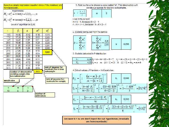
HOMOSCEDASTICITY Harrison-Mc. Cabe test – for models with residuals normally distributed Hypotheses: Statistic from the sample is given by the formula: where: b - Harrison – Mc. Cabe statistic; ei - residuals; n – sample size; m - number of observation (1 < m < n )

HOMOSCEDASTICITY Observation numbered with m should be found in the following way: • m=n/2 if n is an even number or m=(n-1)/2 if n is an odd number, where there’s no tendency in residuals variability, • if absolute residual values are increasing (or decreasing) and than decreasing (or increasing) we should choose for m an observation with the highest (or lowest) residual’s absolute value. We must remember that · m > k +1 · n – m > k + 1 where k – number of estimators.

HOMOSCEDASTICITY Next step is to find F-statistic value at the level of significance and the following number of the degrees of freedom: • F 1 for r 1=n-m and r 2= m-(k+1) df; • F 2 for r 1=n-m-(k+1) and r 2=m df Critical value of Harrison – Mc. Cabe test is given by the formula

HOMOSCEDASTICITY Decision rule: we reject the null hypothesis if The residuals are heteroscedastic we don’t reject the null hypothesis if The residuals are homoscedastic we can’t make any decision (the test is inconclusive) if

AUTOCORRELATION In this section we will examine the effects on the regression model if the error terms in a regression model are correlated with one another. Up to this point we have assumed that the random errors for our model are independent. However, in many business and economic problems we use time series data. When time series data are analyzed, the error term represents the effect of all factors other than the independent variables, that influence the dependent variable. In time series data the behavior of many of these factors might be quite similar over several time periods and the result would be a correlation between the error terms that are close together in time.

AUTOCORRELATION The classical regression model includes an assumption about the independence of the disturbances from observation to observation: E(eiej)=0 for i j [the variance-covariance matrix is diagonal] If this assumption is violated the errors in one time period are correlated with their own values in other periods and there is the problem of autocorrelation - also sometimes referred to as serial correlation - strictly autocorrelated errors or disturbances. All time series variables can exhibit autocorrelation, with the values in a given period depending on values of the same series in previous periods. But the problem of autocorrelation concerns such dependence in the disturbances.

AUTOCORRELATION First order autocorrelation In its simplest form the errors or disturbances in one period are related to those in the previous period by a simple first-order autoregressive process: et = et-1 + t -1 < < 1 If > 0 we have positive autocorrelation, with each error arising as a proportion of last period's error plus a random shock (or innovation). If < 0 it corresponds to negative autocorrelation.

AUTOCORRELATION We shall begin by assuming that any autocorrelation in the errors follows such a first order process. We would say that e is AR(1). Later, however, we must consider the possibility that the errors follow an AR(p) process where p>1 , i. e. et = 1 et-1 + 2 et-2 +. . . . + pet-p + t

AUTOCORRELATION The sources of autocorrelation Each of the following types of misspecification can result in autocorrelated disturbances: Ø incorrect functional form Ø inappropriate time periods Ø inappropriately "filtered" data (seasonal adjustment)

AUTOCORRELATION The consequences of autocorrelation The variances of the parameter estimates will be affected. Consequently the standard errors of the parameter estimators and t -values will also be affected. The variance of the error (Se 2) term will be underestimated so that R squared will be exaggerated. The F-test formulae will also be incorrect.

AUTOCORRELATION Detecting autocorrelation - graphical method

AUTOCORRELATION Detecting autocorrelation –the Durbin-Watson test [J. Durbin and G. S. Watson "Testing for Serial Correlation in Least Squares Regression" Biometrika 1950 and 1951] This test is only appropriate against AR(1) errors. It tests the hypothesis of = 0 in the process et = et-1 + t H 0 : = 0 [no autocorrelation] H 1 : > 0 [or <0 if you are testing for negative autocorrelation] The test statistic is calculated by: et are the residuals when the regression equation is estimated by OLS. d (or DW) can range between 0 and 4.

AUTOCORRELATION It can be shown that So with zero autocorrelation ( = 0 ) we expect d = 2 with positive autocorrelation (0< <1) we expect 0<d<2 with negative autocorrelation (-1< <0) we expect 2<d<4 Thus the test = 0 is a test of d=2.

AUTOCORRELATION The test of the null hypothesis of no autocorrelation H 0: ρ=0 vs. H 1: ρ>0 (positive autocorrelation in errors) is based on the Durbin-Watson statistic Reject Ho if d < d. L where d. L and d. U are tabulated Do not reject Ho if d > d. U Test inconclusive if d. L < d. U for values of n and k and for significance levels of 1% and 5%.

AUTOCORRELATION Occasionally, one wants to test against the alternative of negative autocorrelation that is H 1: ρ<0 the decision rule is as follows: Reject Ho if d > 4 - d. L Do not reject Ho if d < 4 - d. U Test inconclusive if 4 - d. L > d > 4 - d. U

AUTOCORRELATION where d. L and d. U are tabulated for values of n and k and for significance levels of 1% and 5%.

AUTOCORRELATION

SYMMETRY The number of positive actual values differing in plus (in minus) from the fitted values should be a half of all observation (in probability sense). It means that the regression model should be an axis of the symmetry of the dependent variable.

SYMMETRY

DESIRED PROPERTIES OF RESIDUALS Linearity (Don’t reject H 0 in runs test) Normality (Don’t reject H 0 in JB test) Homoscedasticity (Don’t reject H 0 in Harrison-Mc. Cabe test) Symmetry (Don’t reject H 0 in t-Student test) No autocorrelation (Don’t reject H 0 in Durbin-Watson test)

MULTICOLLINEARITY This refers to the situation where one (collinearity) or more (multicollinearity) of the independent variables can be predicted almost exactly from the remainder of the set. In this case, the independent variable set is obviously redundant (redundant – not necessary because sth else means the same) in some sense. If the independent variables are multicollinear, the regression coefficients we calculate will be very unstable - they will vary markedly from sample to sample - so it will be difficult to decide correctly which are the important regressors.

MULTICOLLINEARITY Thus multicollinearity is condition that occurs when two or more of the independent variables of a multiple regression model are highly correlated. • difficult to interpret the estimates of the regression coefficients • inordinately small t values for the regression coefficients may result • standard deviations of regression coefficients are overestimated • sign of predictor variable’s coefficient opposite of what expected

MULTICOLLINEARITY If a regression model is correctly specified and the assumptions are satisfied the least squares estimates are the best that can be achieved. Nevertheless, in some circumstances, they may not be very good! One very bad choice would be to choose independent variables that are highly correlated. It is impossible to estimate the coefficients if the independent variables were perfectly correlated. Suppose we were attempting to use independent correlated variables values such as these to estimate the coefficients of the regression model

MULTICOLLINEARITY The futility of such a task is apparent. If a change in x 1 occurs simultaneously with a change in x 2 then we cannot tell which of the independent variables actually is related to the change in Y. If we want to assess the separate effects of the independent variables, it is essential that they do not move in unison through the experiment. The standard assumptions for multiple regression analysis exclude cases of this sort.

MULTICOLLINEARITY Multicollinearity and singularity are issues which are derived from the having a correlation matrix with too high of correlation between variables. Multicollinearity is when variables are highly correlated and singularity is when the variables are perfectly correlated. Multicollinearity and singularity expose the redundancy of variables and the need to remove variables from the analysis. Multicollinearity and singularity can cause both logical and statistical problems. Logically, The redundant statistical variables problems weaken related to the analysis. singularity and multicollinearity are related to matrix stability and ability for matrix inversion.

MULTICOLLINEARITY With multicollinearity the effects are additive, the independent variables are inter-related, yet effecting the dependent variable differently. The high the multicollinearity, the greater the difficulty in partitioning out the individual effects of independent variables. Accordingly, the partial regression coefficients are unstable and unreliable.

MULTICOLLINEARITY • High correlation between explanatory variables • Coefficient of multiple determination measures combined effect of the correlated explanatory variables • No new information provided • Leads to unstable coefficients (large standard error) • Depending on the explanatory variables

MULTICOLLINEARITY • Is the degree of correlation between Xs. • A high degree of multicollinearity produces unacceptable uncertainty (large variance) in regression coefficient estimates (i. e. , large sampling variation) • Specifically, the coefficients can change drastically depending on which terms are in or out of the model and also the order they are placed in the model. • It affects interpretation of slopes (variable contribution).

MULTICOLLINEARITY Multicolinearity lead to: Ø Imprecise estimates of slopes and even the signs of the coefficients may be misleading, Ø t-tests which fail to reveal significant factors.

MULTICOLLINEARITY Indicators of multicollinearity: 1. Examine a simple correlation matrix of the independent variables to determine if any of the independent variables are individually correlated. The independent variables themselves are not highly correlated. The only questionable variable might be X 1 and X 2.

MULTICOLLINEARITY Indicators of multicollinearity: 2. Another indication of the likely presence of multicollinearity occurs when, taken as a group, a set of independent variables appears to exert considerable influence on the dependent variable, but when looked at separately, through tests of hypotheses, all appear individually to be insignificant. In this case a linear function of the several variables might be used to compute a new variable to replace several correlated variables.

OUTLIERS Outliers are extreme cases on one variable, or a combination of variables, which have a strong influence on the calculation of statistics. The following box plot provides an example of outliers. Outliers are points which lie far from the main distributions or the main trends of one or more variables.

OUTLIERS Graphical methods for identifying outliers (for simple regression): Observe the scatter plot to identify cases that lie too far from the main distribution.

OUTLIERS Graphical methods for identifying multivariate outliers: Observe the residuals to identify cases for which there is a poor fit between obtained and predicted dependent variable scores. A residuals plot will isolate cases which are outliers.

OUTLIERS Reasons for outliers: • incorrect data entry, • case not a member of intended sample population, • actual distribution of the population has more extreme cases than a normal distribution. Reducing the influence of outliers: • check the data for the case, ensure proper data entry • check if one variable is responsible for most of the outliers, consider deletion of the variable, • delete the case if it is not part of the population, if variables are from population, yet to remain in the analysis, transform the variable to reduce influence.

OUTLIERS Serious outliers should be dealt with as follows: 1. Temporarily remove the observations from the data set; 2. Repeat the regression and see whether the same qualitative results are obtained (the quantitative results will inevitably be different). ØIf the same general results are obtained, we can conclude that the outliers are not distorting the results. Report the results of the original regression, adding a note that removal of outliers did not greatly affect them. ØIf different general results are obtained, accurate interpretation will require more data to be collected. Report the results of both regressions, and note that the interpretation of the data is uncertain. The outliers may represent a subpopulation for which the effects of interest are different from those in the main population; this group will need to be identified, and if possible a reasonably sized sample collected from it so that it can be compared with the main population. This is a scientific rather than a statistical problem.