Solving the Graph-partitioning Problem with Heuristic Search Ariel

Solving the Graph-partitioning Problem with Heuristic Search Ariel Felner Bar-Ilan University Ramat-Gan ISRAEL 1

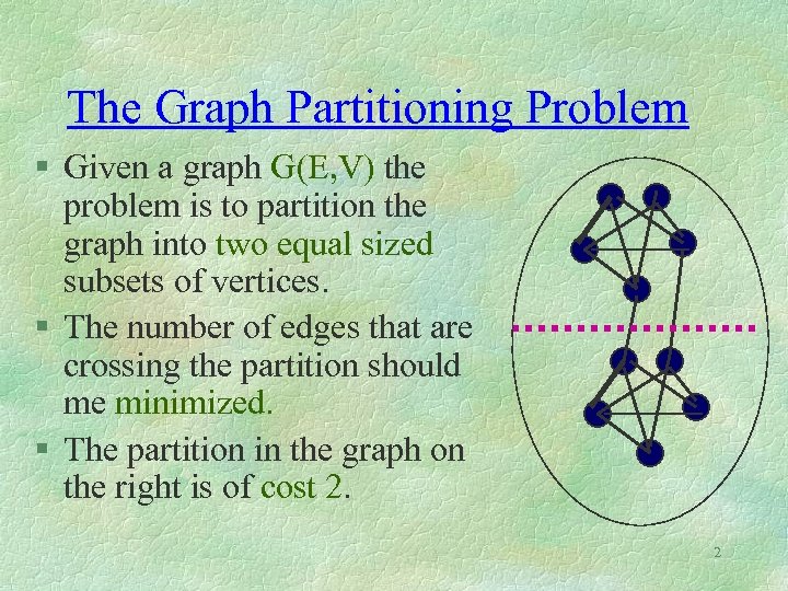
The Graph Partitioning Problem § Given a graph G(E, V) the problem is to partition the graph into two equal sized subsets of vertices. § The number of edges that are crossing the partition should me minimized. § The partition in the graph on the right is of cost 2. 2

Related Work for the GPP § The GPP is NP-Complete. § Most Algorithms for GPP are designed for finding sub-optimal solutions and use local search techniques. § A large portion of them, start with a feasible solution and then start swapping pairs of vertices between the two partitions. § The famous ones are KL (1970) and XLS(1991). 3

A Search Problem § A search space consists states and operators, an initial state, set of goal states. § A solution: a path from the initial state to one of the goal states. § Optimal solution: A path of minimal cost. § Best-first search algorithm: sorts all generated nodes in an OPEN-LIST and chooses the node with the best heuristic value (cost) for expansion. 4

Search Algorithms criteria § Solution quality: Optimal , Near optimal, or Sub optimal. § Time Complexity: number of generated nodes. § Constant time per node: time spent in each node 5

Heuristic functions § Heuristic function: A function that gives each state an estimation of the real distance (cost) from that state to the goal. § A heuristic function is admissible if it never over estimates the real distance. § An admissible heuristic is always a lower bound on the real solution. § Example: air distance in road navigation. § A heuristic function should be as accurate as possible and as fast as possible to 6 compute.

The A* algorithm § g(x): real distance from the initial state to the current node x. § h(x): the estimated remained distance from x to the goal state. § f(x)=g(x): Uniform Cost Search. § f(x)=g(x)+h(x): The A* algorithm (1968). § f(x) in A* is an estimation of the shortest path to the goal via x. § Theorem: “Given a heuristic function, no other algorithm outperforms A*”. (Pearl 83). 7

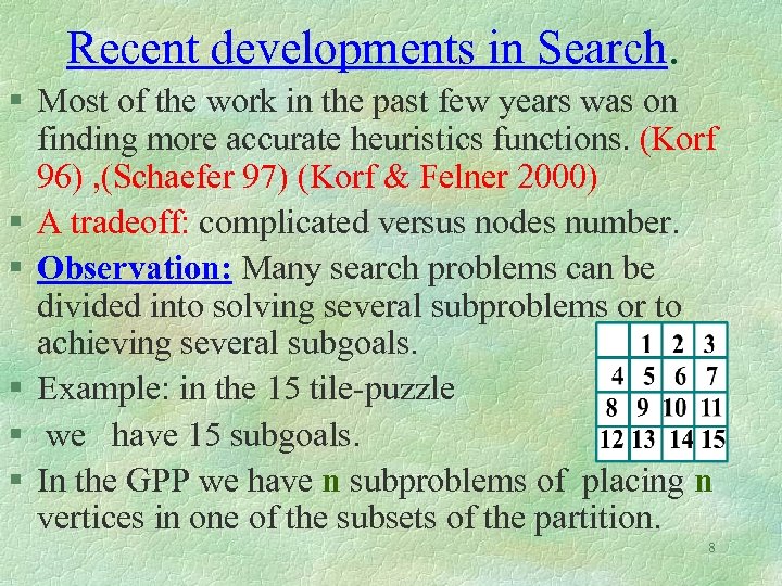
Recent developments in Search. § Most of the work in the past few years was on finding more accurate heuristics functions. (Korf 96) , (Schaefer 97) (Korf & Felner 2000) § A tradeoff: complicated versus nodes number. § Observation: Many search problems can be divided into solving several subproblems or to achieving several subgoals. § Example: in the 15 tile-puzzle § we have 15 subgoals. § In the GPP we have n subproblems of placing n vertices in one of the subsets of the partition. 8

Our main hypothesis § Our claim: ”Looking more deeply into interactions between unsolved sub goals resolves with a much better heuristic function and speeds up the search” 9

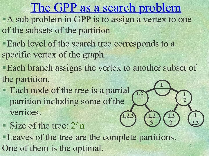
The GPP as a search problem § A sub problem in GPP is to assign a vertex to one of the subsets of the partition § Each level of the search tree corresponds to a specific vertex of the graph. § Each branch assigns the vertex to another subset of the partition. 1 § Each node of the tree is a partial 1, 2 1 2 partition including some of the vertices. 1 1, 2, 3 1, 2 1, 3 3 2 2, 3 § Size of the tree: 2^n § Leaves of the tree are the complete partitions. 10 One of them is the optimal.

Definitions § A node of the search tree is denoted by k while vertex of the graph is denoted by x. § A vertex that is already assigned to one of the subsets is called an assigned vertex. § Each of the other vertices is a free vertex. Free vertices are unsolved subgoals. § Given a node k of the search tree we define: g(k): the number of edges that already cross the partial partition due to assigned vertices. h(k): A lower bound on the number of edges that will cross the given partition due to free vertices. 11

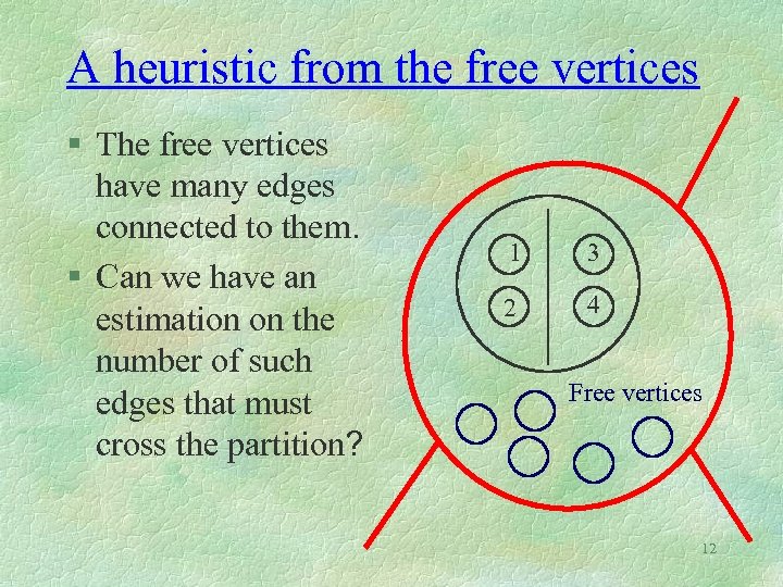
A heuristic from the free vertices § The free vertices have many edges connected to them. § Can we have an estimation on the number of such edges that must cross the partition? 1 3 2 4 Free vertices 12

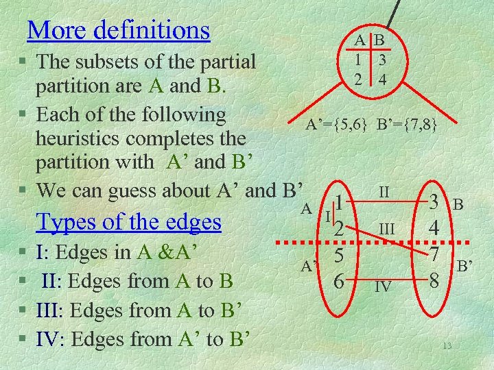
More definitions A B 1 3 2 4 § The subsets of the partial partition are A and B. § Each of the following A’={5, 6} B’={7, 8} heuristics completes the partition with A’ and B’ II § We can guess about A’ and B’ 3 B A I 1 Types of the edges III 4 2 § I: Edges in A &A’ 7 B’ 5 A’ 8 § II: Edges from A to B 6 IV § III: Edges from A to B’ § IV: Edges from A’ to B’ 13

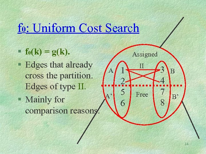
f 0: Uniform Cost Search § f 0(k) = g(k). § Edges that already cross the partition. Edges of type II. § Mainly for comparison reasons. Assigned A A’ 1 2 5 6 II Free 3 4 7 8 B B’ 14

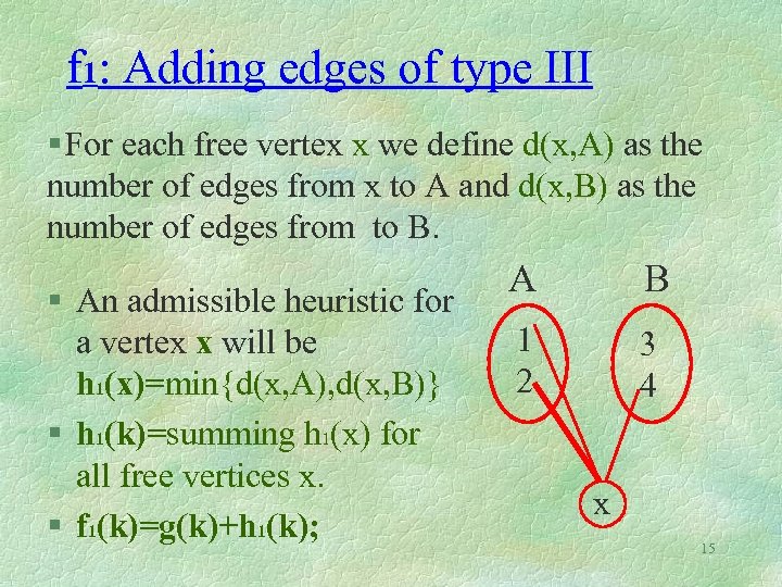
f 1: Adding edges of type III § For each free vertex x we define d(x, A) as the number of edges from x to A and d(x, B) as the number of edges from to B. § An admissible heuristic for a vertex x will be h 1(x)=min{d(x, A), d(x, B)} § h 1(k)=summing h 1(x) for all free vertices x. § f 1(k)=g(k)+h 1(k); A B 1 2 3 4 x 15

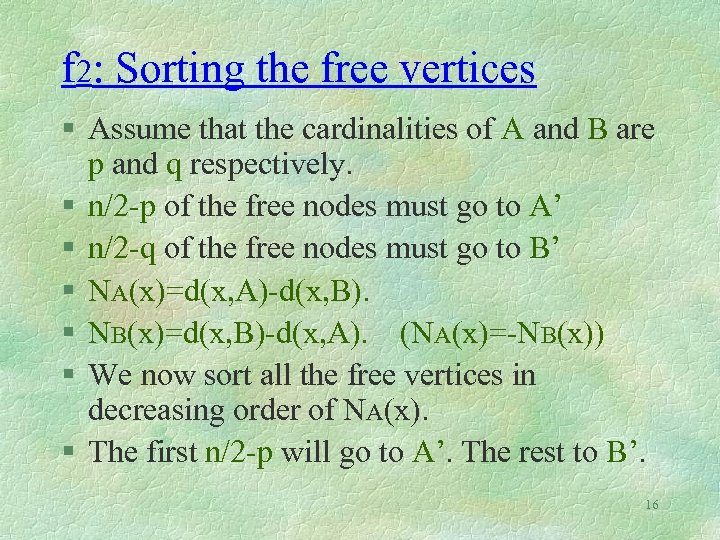
f 2: Sorting the free vertices § Assume that the cardinalities of A and B are p and q respectively. § n/2 -p of the free nodes must go to A’ § n/2 -q of the free nodes must go to B’ § NA(x)=d(x, A)-d(x, B). § NB(x)=d(x, B)-d(x, A). (NA(x)=-NB(x)) § We now sort all the free vertices in decreasing order of NA(x). § The first n/2 -p will go to A’. The rest to B’. 16

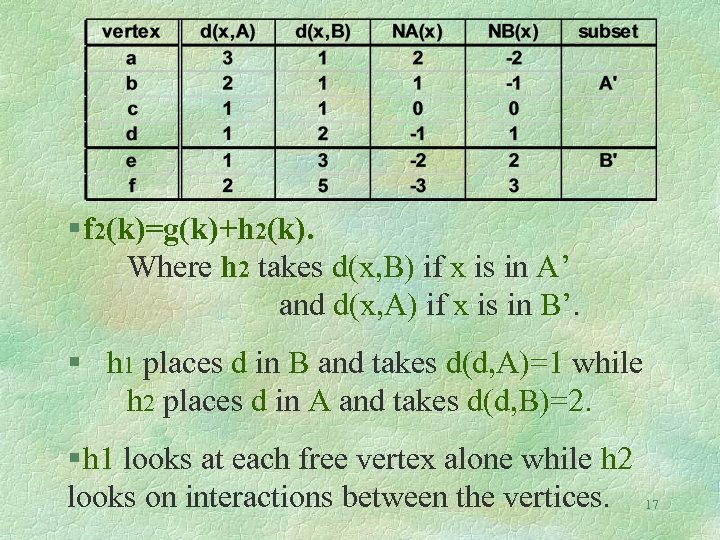
§ f 2(k)=g(k)+h 2(k). Where h 2 takes d(x, B) if x is in A’ and d(x, A) if x is in B’. § h 1 places d in B and takes d(d, A)=1 while h 2 places d in A and takes d(d, B)=2. § h 1 looks at each free vertex alone while h 2 looks on interactions between the vertices. 17

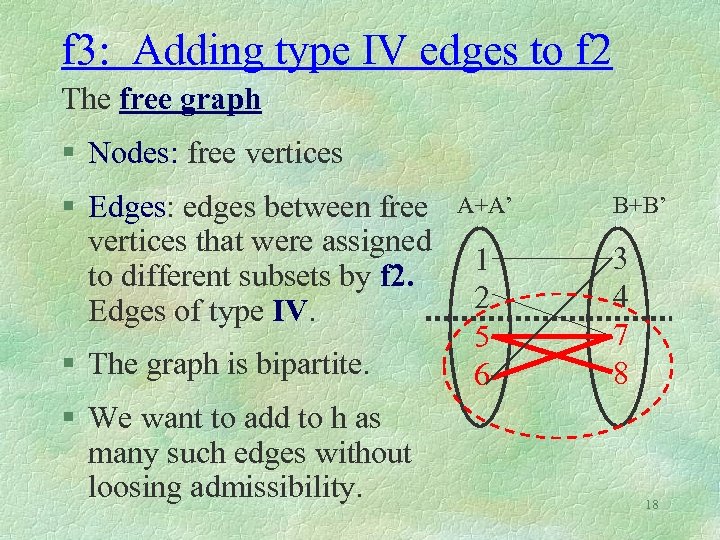
f 3: Adding type IV edges to f 2 The free graph § Nodes: free vertices § Edges: edges between free vertices that were assigned to different subsets by f 2. Edges of type IV. § The graph is bipartite. § We want to add to h as many such edges without loosing admissibility. A+A’ 1 2 5 6 B+B’ 3 4 7 8 18

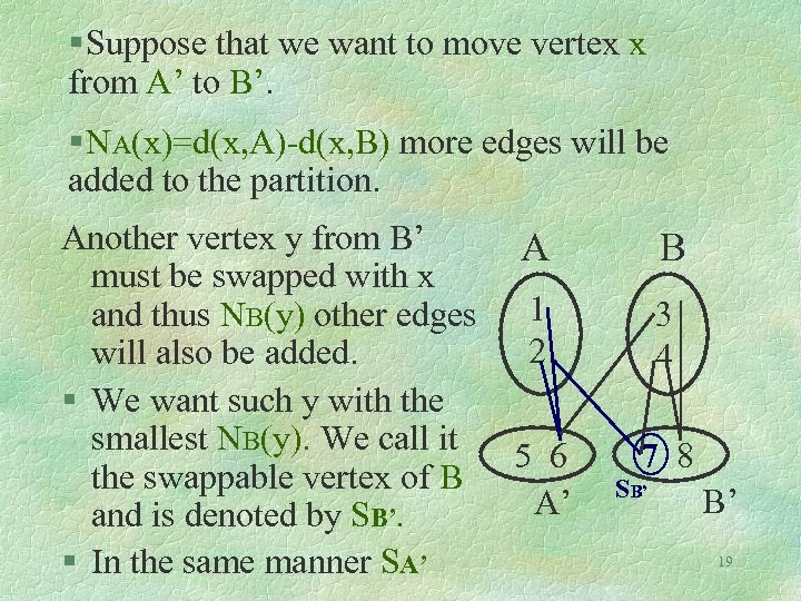
§ Suppose that we want to move vertex x from A’ to B’. § NA(x)=d(x, A)-d(x, B) more edges will be added to the partition. Another vertex y from B’ must be swapped with x and thus NB(y) other edges will also be added. § We want such y with the smallest NB(y). We call it the swappable vertex of B and is denoted by SB’. § In the same manner SA’ A B 1 2 3 4 5 6 A’ 7 8 SB’ B’ 19

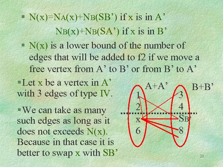
§ N(x)=NA(x)+NB(SB’) if x is in A’ NB(x)+NB(SA’) if x is in B’ § N(x) is a lower bound of the number of edges that will be added to f 2 if we move a free vertex from A’ to B’ or from B’ to A’ § Let x be a vertex in A’ A+A’ B+B’ with 3 edges of type IV. 3 1 4 2 § We can take as many SB’ x such edges as long as it 8 6 does not exceeds N(x). Because in that case it is better to swap x with SB’ 20

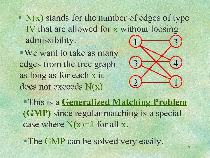
§ N(x) stands for the number of edges of type IV that are allowed for x without loosing admissibility. 1 3 § We want to take as many 3 4 edges from the free graph as long as for each x it 2 1 does not exceeds N(x) § This is a Generalized Matching Problem (GMP) since regular matching is a special case where N(x)=1 for all x. § The GMP can be solved very easily. 21

Summary of f 3 § f 3(k)=g(k)+h 2(k)+h 3(k). § 1) Sort the free vertices in decreasing order of NA(x). § 2) calculate h 2 for each of the free vertices. § 3) Identify the swappable vertices and for each free vertex x calculate N(x). § 4) Form the GMP with N(X). § 5) Calculate h 3 by solving the GMP. 22

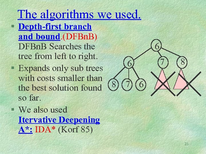
The algorithms we used. § Depth-first branch and bound. (DFBn. B) DFBn. B Searches the tree from left to right. § Expands only sub trees with costs smaller than the best solution found 8 so far. § We also used Itervative Deepening A*: IDA* (Korf 85) 6 6 7 8 7 6 23

Empirical results § Given the size of the graph n and a branching factor b, we built a random graph with n nodes and each edge was added to the graph with a probability of b/n. § The nodes of the graph were sorted by decreasing order of their branching factor and thus nodes with more edges will be treated sooner. § Experiments were done on a 500 MHZ pc. § Data was averaged on 30 similar datapoints 24

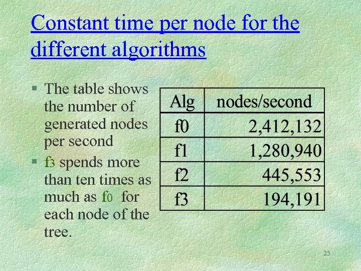
Constant time per node for the different algorithms § The table shows the number of generated nodes per second § f 3 spends more than ten times as much as f 0 for each node of the tree. 25

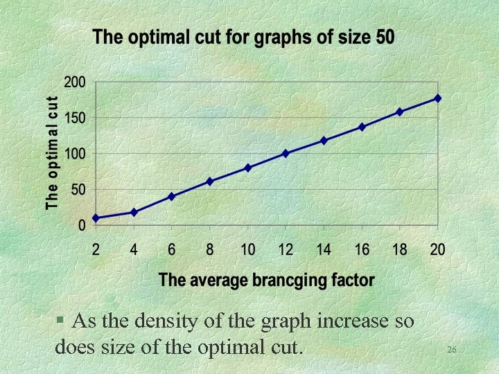
§ As the density of the graph increase so does size of the optimal cut. 26

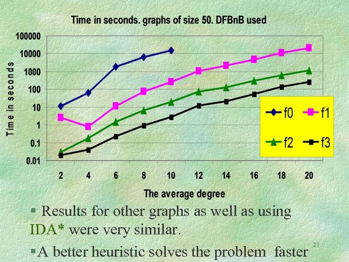
§ Results for other graphs as well as using IDA* were very similar. 27 § A better heuristic solves the problem faster

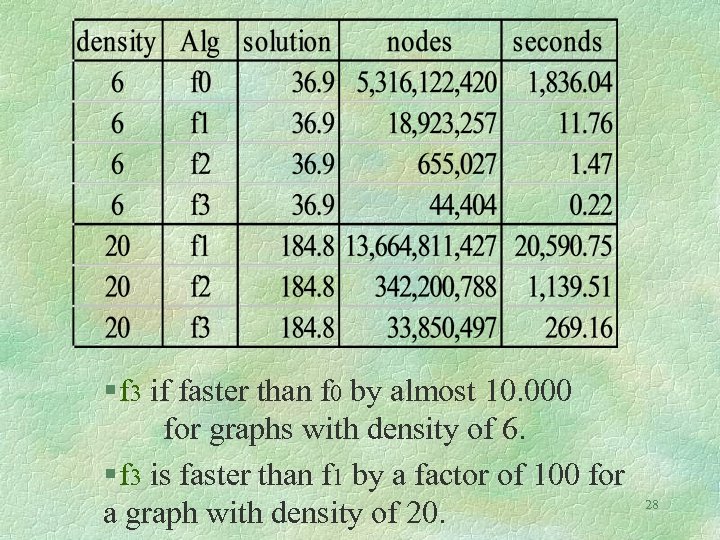
§ f 3 if faster than f 0 by almost 10. 000 for graphs with density of 6. § f 3 is faster than f 1 by a factor of 100 for a graph with density of 20. 28

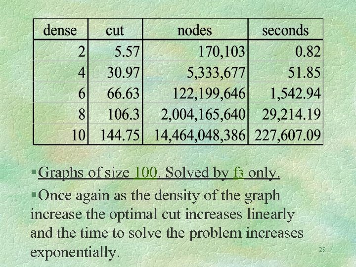
§ Graphs of size 100. Solved by f 3 only. § Once again as the density of the graph increase the optimal cut increases linearly and the time to solve the problem increases exponentially. 29

Discussion § Our approach can be combined with any other sub optimal algorithm A, by first running A and then giving its solution as a bound to DFBn. B. § (Rolland Pirkul 99) developed an algorithm that finds the size of the optimal solution very quickly based on Lagrangian relaxation and subgradient search. § The threshold for both IDA* and DFBn. B can come from their method. 30

Conclusions. § We have shown an algorithm that finds optimal solution to the GPP. § We have demonstrated the claim that finding better heuristics by looking deeply into interactions between subgoals speeds up the search. § We have developed similar heuristics to the Vertex Cover problem and the Sliding tile puzzles with again nice speedup. 31