Software Synthesis using Automated Reasoning Ruzica Piskac SVARM

Software Synthesis using Automated Reasoning Ruzica Piskac SVARM 2011 Saarbrücken, Germany 1

specification (formula) automated reasoning (theorem prover) code SOFTWARE SYNTHESIS 2

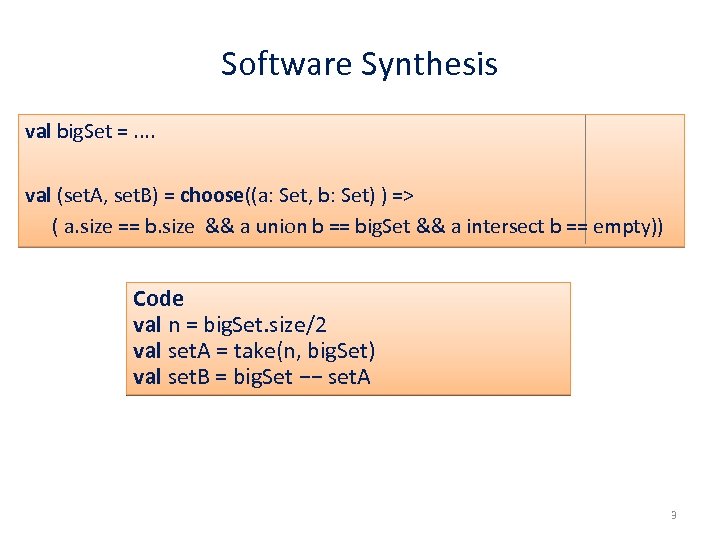Software Synthesis val big. Set =. . val (set. A, set. B) = choose((a: Set, b: Set) ) => ( a. size == b. size && a union b == big. Set && a intersect b == empty)) Code val n = big. Set. size/2 val set. A = take(n, big. Set) val set. B = big. Set −− set. A 3

Software Synthesis val big. Set =. . val (set. A, set. B) = choose((a: Set, b: Set) ) => ( a. size == b. size && a union b == big. Set && a intersect b == empty)) Code assert (big. Set. size % 2 == 0) val n = big. Set. size/2 val set. A = take(n, big. Set) val set. B = big. Set −− set. A 4

Software Synthesis • Software synthesis = a technique for automatically generating code given a specification • Why? – ease software development – increase programmer productivity – fewer bugs • Challenges – synthesis is often a computationally hard task – new algorithms are needed 5

Software Synthesis – Then and Now • Studied for a long time – Church Synthesis Problem – Zohar Manna, Richard J. Waldinger: “A Deductive Approach to Program Synthesis” [1980] • Recent increased interests – due to increasing computational power and improvements in automated reasoning – Sumit Gulwani (MSR): search-based techniques – Ras Bodik (Berkley): Programming by Sketching 6

COMPLETE FUNCTIONAL SYNTHESIS JOINT WORK WITH VIKTOR KUNCAK, MIKAEL MAYER AND PHILIPPE SUTER [PLDI 2010, CAV 2010, CACM 2011/2] 7

Synthesis as programming language construct … val x = read. Integer() + 4 val y 1 = choose(y ⇒ 5*x + 7*y == 31) println(“y 1 = “ + y 1) … 8

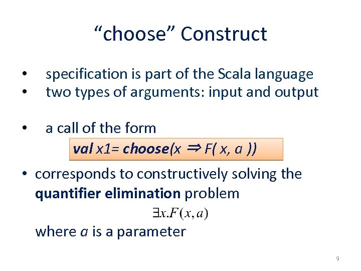“choose” Construct • • specification is part of the Scala language two types of arguments: input and output • a call of the form val x 1= choose(x ⇒ F( x, a )) • corresponds to constructively solving the quantifier elimination problem where a is a parameter 9

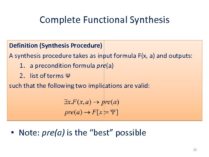Complete Functional Synthesis Definition (Synthesis Procedure) A synthesis procedure takes as input formula F(x, a) and outputs: 1. a precondition formula pre(a) 2. list of terms Ψ such that the following two implications are valid: • Note: pre(a) is the “best” possible 10

From Decision Procedure to Synthesis Procedure • based on quantifier elimination / model generating decision procedures • implemented for logic of linear integer (rational, real) arithmetic, for Boolan Algebra with Presburger Arithmetic (BAPA) 11

Complete Functional Synthesis • • • – – complete = the synthesis procedure is guaranteed to find code that satisfies the given specification functional = computes a function that satisfies a given input / output relation Important features: code produced this way is correct by construction – no need for further verification a user does not provide hints on the structure of the generated code 12

Synthesis for Linear Integer Arithmetic – Example / Overview choose((h: Int, m: Int, s: Int) ⇒ ( h * 3600 + m * 60 + s == total. Seconds && h ≥ 0 && m < 60 && s ≥ 0 && s < 60 )) Returned code: assert (total. Seconds ≥ 0) val h = total. Seconds div 3600 val temp = total. Seconds + (-3600) * h val m = temp div 60 val s = total. Seconds + (-3600) * h + (-60)* m 13

Synthesis Procedure - Overview • process every equality: take an equality Ei, compute a parametric description of the solution set and insert those values in the rest of formula – for n output variables, we need n-1 fresh new variables – number of output variables decreased for 1 – based on Extended Euclidean Algorithm – compute preconditions 14

Synthesis Procedure - Overview • at the end there are only inequalities – similar procedure as in [Pugh 1992] 15

Parametric Solution of Equation Theorem For an equation • with S we denote the set of solutions. Let SH be a set of solutions of the homogeneous equality: SH = { y | } SH is an “almost linear” set, i. e. can be represented as a linear combination of vectors: SH = λ 1 s 1 +. . . λn-1 sn-1 • Let w be any solution of the original equation • S = w + λ 1 s 1 +. . . λn-1 sn-1 + preconditions: gcd( i)| C 16

Solution of a Homogenous Equation Theorem For an equation with SH we denote the set of solutions. where values Kij are computed as follows: • if i < j, Kij = 0 (the matrix K is lower triangular) • if i =j • for remaining Kij values, find any solution of the equation 17

Finding any Solution (n variables) • Inductive approach – 1 x 1 + 2 x 2 +. . . + nxn = C 1 x 1 + gcd( 2, . . . , n )[λ 2 x 2 +. . . + λnxn] = C 1 x 1 + x. F = C • find values for x 1 (w 1) and x. F (w. F) and then solve inductively: λ 2 x 2 +. . . + λnxn = w. F 18

Finding any Solution (2 variables) • based on Extended Euclidean Algorithm (EEA) – for every two integers n and m finds numbers p and q such that n*p + m*q = gcd(n, m) • problem: 1 x 1 + 2 x 2 = C • solution: – apply EEA to compute p and q such that 1 p + 2 q = gcd( 1, 2) – solution: x 1 = p*C/ gcd( 1, 2) x 2 = q*C/ gcd( 1, 2) 19

Linear Integer Arithemtic: Example val (x 1, y 1) = choose(x: Int, y: Int => 2*y − b =< 3*x + a && 2*x − a =< 4*y + b) val k. Found = false for k = 0 to 5 do { val v 1 = 3 * a + 3 * b − k if (v 1 mod 6 == 0) { val alpha = ((k − 5 * a − 5 * b)/8). ceiling val l = (v 1 / 6) + 2 * alpha val y = alpha val k. Found = true break } } if (k. Found) val x = ((4 * y + a + b)/2). floor else throw new Exception(”No solution exists”) Precondition: ∃k. 0 ≤ k ≤ 5 ∧ 6|3 a + 3 b − k 20

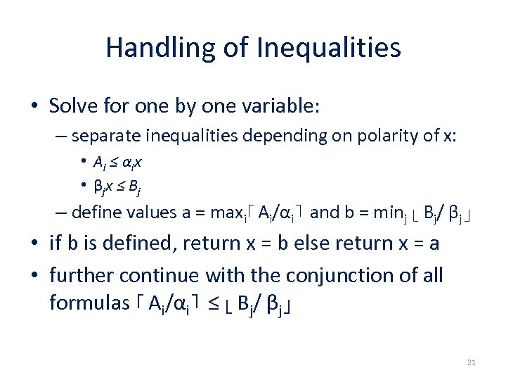Handling of Inequalities • Solve for one by one variable: – separate inequalities depending on polarity of x: • A i ≤ α ix • β jx ≤ B j – define values a = maxi⌈ Ai/αi⌉ and b = minj ⌊ Bj/ βj⌋ • if b is defined, return x = b else return x = a • further continue with the conjunction of all formulas ⌈ Ai/αi⌉ ≤ ⌊ Bj/ βj⌋ 21

Algorithm for more than one Variable Consider the formula 2 y − b ≤ 3 x + a ∧ 2 x − a ≤ 4 y + b ⌈ (2 y − b − a)/3⌉ ≤ ⌊ (4 y + a + b)/2⌋ ⇔ ⌈ (2 y − b − a) ∗ 2/6⌉ ≤ ⌊ (4 y + a + b) ∗ 3/6⌋ ⇔ (4 y − 2 b − 2 a)/6 ≤ [(12 y + 3 a + 3 b) − (12 y + 3 a + 3 b) mod 6]/6 ⇔ (12 y + 3 a + 3 b) mod 6 ≤ 8 y + 5 a + 5 b ⇔ 12 y + 3 a + 3 b = 6 ∗ l + k ∧ k ≤ 8 y + 5 a + 5 b 22

Algorithm for more than one Variable Consider the formula 2 y − b ≤ 3 x + a ∧ 2 x − a ≤ 4 y + b • 12 y + 3 a + 3 b = 6 ∗ l + k ∧ k ≤ 8 y + 5 a + 5 b • upon applying the equality, we obtain – preconditions: 6|3 a + 3 b − k – solutions: l = 2λ + (3 a + 3 b − k)/6 and y = λ • substituting those values in the inequality results in k − 5 a − 5 b ≤ 8λ • final solution: λ = ⌈ (k − 5 a − 5 b)/8⌉ 23

Synthesis for Sets val (set. A, set. B) = choose((a: Set[O], b: Set[O]) ) => (−max. Diff <= a. size − b. size && a. size − b. size <= max. Diff && a union b == big. Set && a intersect b == empty)) Code val k. A = ((big. Set. size + max. Diff)/2). floor val set. A = take(k. A, big. Set) val set. B = big. Set −− set. A Precondition ⌈ |big. Set| − max. Diff/2⌉ ≤ ⌊ |big. Set| + max. Diff/2⌋ 24

INTERACTIVE SYNTHESIS OF CODE SNIPPETS JOINT WORK WITH TIHOMIR GVERO AND VIKTOR KUNCAK [UNDER SUBMISSION, CAV 2011] 25

isynth - Interactive Synthesis of Code Snippets def fopen(name: String): File = {. . . } def fread(f: File, p: Int): Data = {. . . } var current. Pos : Int = 0 var fname : String= null. . . def get. Data(): Data = Returned value: fread(fopen(fname), current. Pos) 26

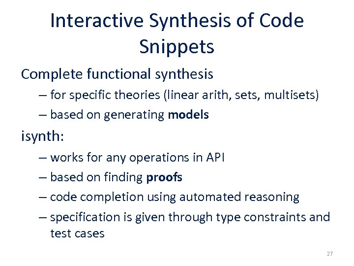Interactive Synthesis of Code Snippets Complete functional synthesis – for specific theories (linear arith, sets, multisets) – based on generating models isynth: – works for any operations in API – based on finding proofs – code completion using automated reasoning – specification is given through type constraints and test cases 27

isynth – Polymorphic Types def map[A, B](f: A => B, l: List[A]): List[B] = {. . . } def string. Concat(lst : List[String]): String = {. . . }. . . def print. Ints(int. List: List[Int], prn: Int => String): String = Returned value: string. Concat(map[Int, String](prn, int. List)) 28

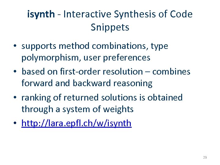isynth - Interactive Synthesis of Code Snippets • supports method combinations, type polymorphism, user preferences • based on first-order resolution – combines forward and backward reasoning • ranking of returned solutions is obtained through a system of weights • http: //lara. epfl. ch/w/isynth 29

System of weights in isynth • Symbol weights Low High User preferred Arrow Method and field symbols Local symbols API symbols • Term weights – Recalculate weight of terms with user preferred symbols 30

isynth - Evaluation Program # Loaded Declarations # Methods in Synthesized Snippets Time [s] File. Reader 5 4 0. 001 Map 3 3 < 0. 001 File. Manager 7 3 0. 001 Calendar 29 3 0. 001 File. Writer 442 6 0. 72 Swing. Border 161 2 0. 02 Tcp. Service 112 3 0. 62 31

Related Work / Reading Material Comfusy project: – M. Mayer, R. Piskac, P. Suter: “Complete Functional Synthesis”, PLDI 2010 – V. Kuncak, M. Mayer, R. Piskac, P. Suter: “Comfusy: A Tool for Complete Functional Synthesis”, CAV 2010 – A. Solar-Lezama, L. Tancau, R. Bodík, S. A. Seshia, V. A. Saraswat: “Combinatorial sketching for finite programs”. ASPLOS 2006 – S. Jha, S. Gulwani, S. A. Seshia, A. Tiwari: “Oracle-guided component-based program synthesis”. ICSE (1) 2010 – S. Srivastava, S. Gulwani, J. S. Foster: From program verification to program synthesis. POPL 2010 – S. Gulwani: Dimensions in program synthesis. PPDP 2010 isynth project: – T. Gvero, R. Piskac, V. Kuncak. “Interactive Synthesis of Code Snippets”, CAV 2011 – The Agda Project [http: //wiki. portal. chalmers. se/agda/] – D. Mandelin, L. Xu, R. Bodık, D. Kimelman: “Jungloid mining: helping to navigate the API jungle”, PLDI '05 32

Conclusions Software Synthesis – method to obtain correct software from the given specification – Complete Functional Synthesis: extending decision procedures into synthesis algorithms – Interactive Synthesis of Code Snippets finding a term of a given type Contributions to/from automated reasoning – decision procedures – methods to combine them 33

SYNTHESIS FOR LINEAR INTEGER ARITHMETIC 34

Quantifier Elimination for Linear Integer Arithmetic • Problem of great interest: – [Presburger, 1929], [Cooper, 1972] – [Pugh, 1992], – [Weispfenning, 1997] – [Nipkow 2008] – verified in Isabelle • Our algorithm for integers: – Efficient handling equalities – Handling of inequalities as in [Pugh 1992] – Computes witness terms , builds a program from 35 them

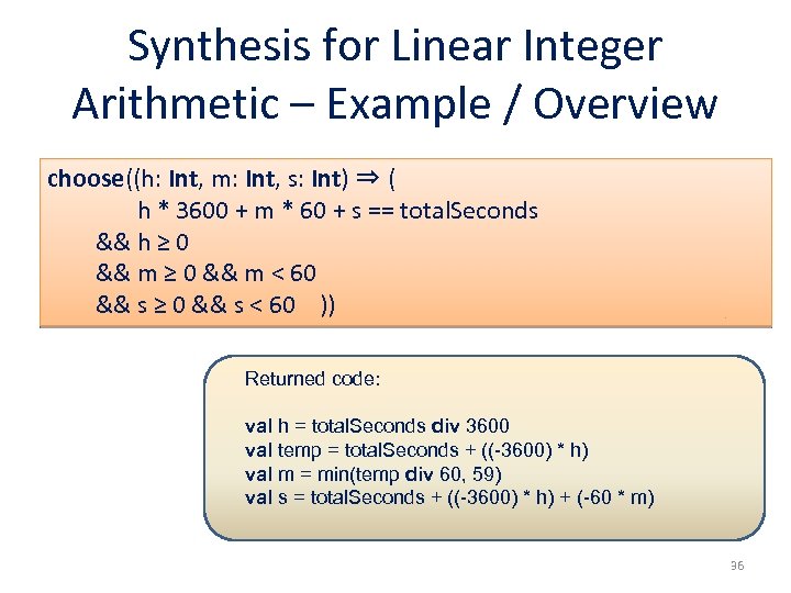Synthesis for Linear Integer Arithmetic – Example / Overview choose((h: Int, m: Int, s: Int) ⇒ ( h * 3600 + m * 60 + s == total. Seconds && h ≥ 0 && m < 60 && s ≥ 0 && s < 60 )) Returned code: val h = total. Seconds div 3600 val temp = total. Seconds + ((-3600) * h) val m = min(temp div 60, 59) val s = total. Seconds + ((-3600) * h) + (-60 * m) 36

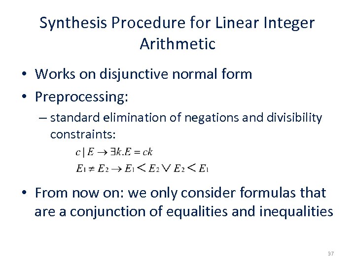Synthesis Procedure for Linear Integer Arithmetic • Works on disjunctive normal form • Preprocessing: – standard elimination of negations and divisibility constraints: • From now on: we only consider formulas that are a conjunction of equalities and inequalities 37

Overview of a Synthesis Procedure 1. process every equality: take an equality Ei, compute a parametric description of the solution set and insert those values in the rest of formula • • • for n output variables, we need n-1 fresh new variables number of output variables decreased for 1 compute preconditions 2. at the end there are only inequalities – same procedure as in [Pugh 1992] 38

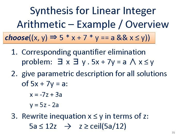Synthesis for Linear Integer Arithmetic – Example / Overview choose((x, y) ⇒ 5 * x + 7 * y == a && x ≤ y)) 1. Corresponding quantifier elimination problem: ∃ x ∃ y. 5 x + 7 y = a ∧ x ≤ y 2. give parametric description for all solutions of 5 x + 7 y = a: x = -7 z + 3 a y = 5 z - 2 a 3. Rewrite inequation x ≤ y in terms of z: 5 a ≤ 12 z → z ≥ ceil(5 a/12) 39

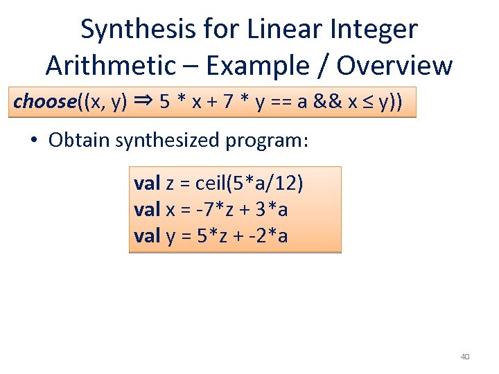Synthesis for Linear Integer Arithmetic – Example / Overview choose((x, y) ⇒ 5 * x + 7 * y == a && x ≤ y)) • Obtain synthesized program: val z = ceil(5*a/12) val x = -7*z + 3*a val y = 5*z + -2*a 40

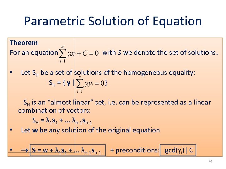Parametric Solution of Equation Theorem For an equation • with S we denote the set of solutions. Let SH be a set of solutions of the homogeneous equality: SH = { y | } SH is an “almost linear” set, i. e. can be represented as a linear combination of vectors: SH = λ 1 s 1 +. . . λn-1 sn-1 • Let w be any solution of the original equation • S = w + λ 1 s 1 +. . . λn-1 sn-1 + preconditions: gcd( i)| C 41

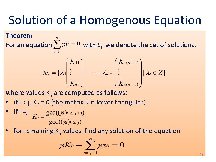Solution of a Homogenous Equation Theorem For an equation with SH we denote the set of solutions. where values Kij are computed as follows: • if i < j, Kij = 0 (the matrix K is lower triangular) • if i =j • for remaining Kij values, find any solution of the equation 42

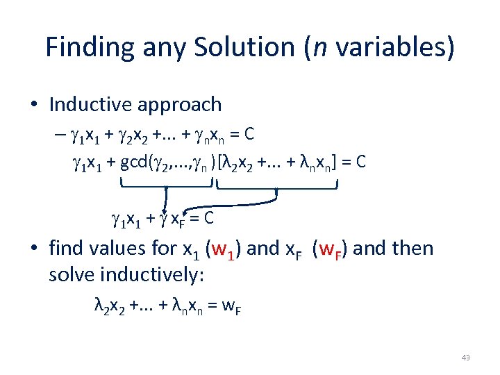Finding any Solution (n variables) • Inductive approach – 1 x 1 + 2 x 2 +. . . + nxn = C 1 x 1 + gcd( 2, . . . , n )[λ 2 x 2 +. . . + λnxn] = C 1 x 1 + x. F = C • find values for x 1 (w 1) and x. F (w. F) and then solve inductively: λ 2 x 2 +. . . + λnxn = w. F 43

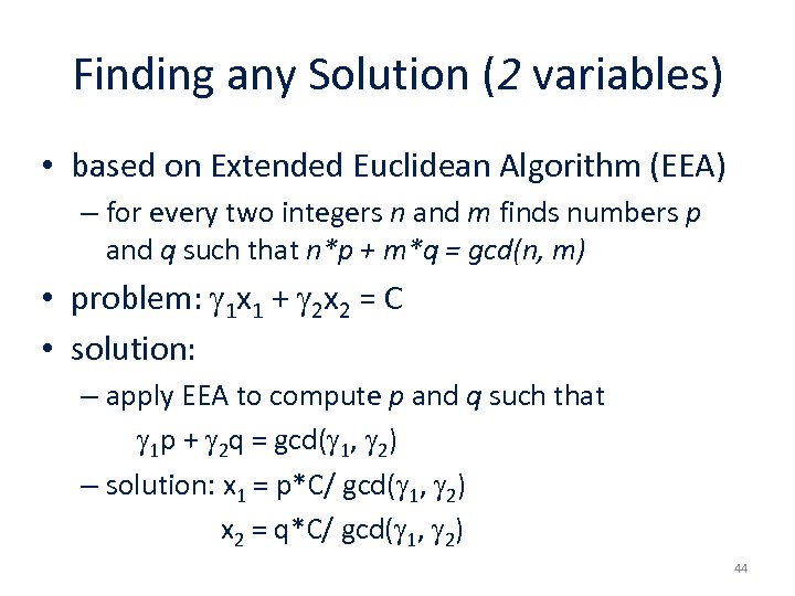Finding any Solution (2 variables) • based on Extended Euclidean Algorithm (EEA) – for every two integers n and m finds numbers p and q such that n*p + m*q = gcd(n, m) • problem: 1 x 1 + 2 x 2 = C • solution: – apply EEA to compute p and q such that 1 p + 2 q = gcd( 1, 2) – solution: x 1 = p*C/ gcd( 1, 2) x 2 = q*C/ gcd( 1, 2) 44

Handling of Inequalities • Solve for one by one variable: – separate inequalities depending on polarity of x: • A i ≤ α ix • β jx ≤ B j – define values a = maxi⌈ Ai/αi⌉ and b = minj ⌊ Bj/ βj⌋ • if b is defined, return x = b else return x = a • further continue with the conjunction of all formulas ⌈ Ai/αi⌉ ≤ ⌊ Bj/ βj⌋ 45

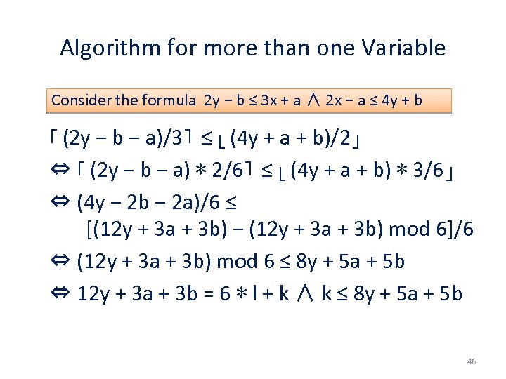Algorithm for more than one Variable Consider the formula 2 y − b ≤ 3 x + a ∧ 2 x − a ≤ 4 y + b ⌈ (2 y − b − a)/3⌉ ≤ ⌊ (4 y + a + b)/2⌋ ⇔ ⌈ (2 y − b − a) ∗ 2/6⌉ ≤ ⌊ (4 y + a + b) ∗ 3/6⌋ ⇔ (4 y − 2 b − 2 a)/6 ≤ [(12 y + 3 a + 3 b) − (12 y + 3 a + 3 b) mod 6]/6 ⇔ (12 y + 3 a + 3 b) mod 6 ≤ 8 y + 5 a + 5 b ⇔ 12 y + 3 a + 3 b = 6 ∗ l + k ∧ k ≤ 8 y + 5 a + 5 b 46

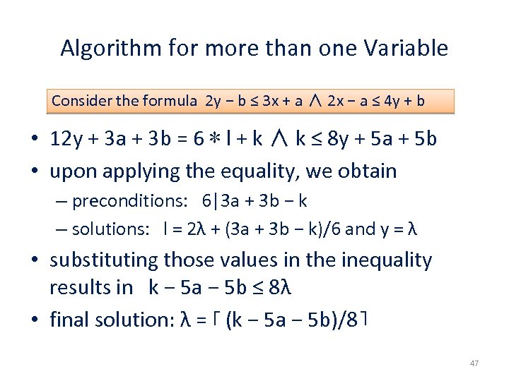Algorithm for more than one Variable Consider the formula 2 y − b ≤ 3 x + a ∧ 2 x − a ≤ 4 y + b • 12 y + 3 a + 3 b = 6 ∗ l + k ∧ k ≤ 8 y + 5 a + 5 b • upon applying the equality, we obtain – preconditions: 6|3 a + 3 b − k – solutions: l = 2λ + (3 a + 3 b − k)/6 and y = λ • substituting those values in the inequality results in k − 5 a − 5 b ≤ 8λ • final solution: λ = ⌈ (k − 5 a − 5 b)/8⌉ 47

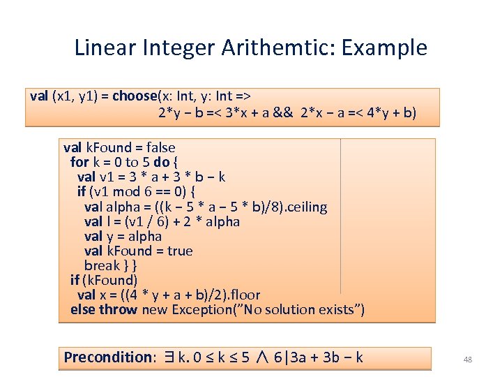Linear Integer Arithemtic: Example val (x 1, y 1) = choose(x: Int, y: Int => 2*y − b =< 3*x + a && 2*x − a =< 4*y + b) val k. Found = false for k = 0 to 5 do { val v 1 = 3 * a + 3 * b − k if (v 1 mod 6 == 0) { val alpha = ((k − 5 * a − 5 * b)/8). ceiling val l = (v 1 / 6) + 2 * alpha val y = alpha val k. Found = true break } } if (k. Found) val x = ((4 * y + a + b)/2). floor else throw new Exception(”No solution exists”) Precondition: ∃k. 0 ≤ k ≤ 5 ∧ 6|3 a + 3 b − k 48

Synthesis for Sets val (set. A, set. B) = choose((a: Set[O], b: Set[O]) ) => (−max. Diff <= a. size − b. size && a. size − b. size <= max. Diff && a union b == big. Set && a intersect b == empty)) Code val k. A = ((big. Set. size + max. Diff)/2). floor val k. B = big. Set. size − k. A val set. A = take(k. A, big. Set) val set. B = take(k. B, big. Set −− set. A) Precondition ⌈ |big. Set| − max. Diff/2⌉ ≤ ⌊ |big. Set| + max. Diff/2⌋ 49

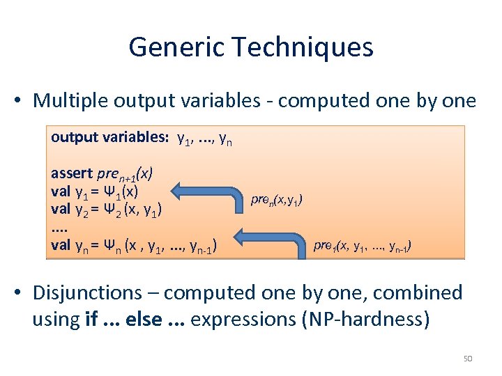Generic Techniques • Multiple output variables - computed one by one output variables: y 1, . . . , yn assert pren+1(x) val y 1 = Ψ 1(x) val y 2 = Ψ 2 (x, y 1). . val yn = Ψn (x , y 1, . . . , yn-1) pren(x, y 1) pre 1(x, y 1, . . . , yn-1) • Disjunctions – computed one by one, combined using if. . . else. . . expressions (NP-hardness) 50