Software Estimation Alberto Sangiovanni Vincentelli Thanks to Prof

Software Estimation Alberto Sangiovanni. Vincentelli Thanks to Prof. Sharad Malik at Princeton University and Prof. Reinhard Wilhelm at Universitat des Saarlandes for some of the slides

Outline u. SW estimation overview u. Program path analysis u. Micro-architecture modeling u. Implementation examples: Cinderella u. SW estimation in VCC u. SW estimation in AI u. SW estimation in POLIS 2

SW estimation overview u. SW estimation problems in HW/SW co-design s The structure and behavior of synthesized programs are known in the co-design system s Quick (and as accurate as possible) estimation methods are needed Quick methods for HW/SW partitioning [Hu 94, Gupta 94] t Accurate method using a timing accurate co-simulation [Henkel 93] t 3

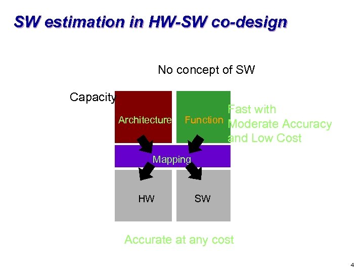
SW estimation in HW-SW co-design No concept of SW Capacity Architecture Fast with Function Moderate Accuracy and Low Cost Mapping HW SW Accurate at any cost 4

SW estimation overview: motivation u SW estimation helps to s Evaluate HW/SW trade-offs s Check performance/constraints t s Higher reliability Reduce system cost t Allow slower hardware, smaller size, lower power consumption 5

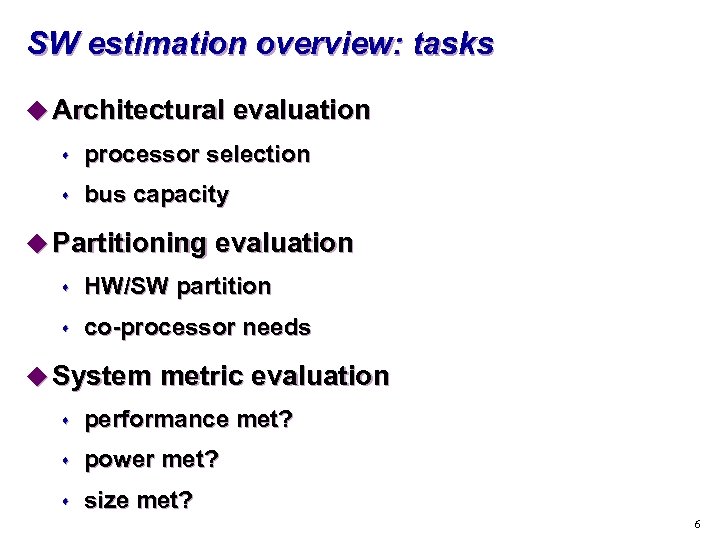
SW estimation overview: tasks u Architectural evaluation s processor selection s bus capacity u Partitioning evaluation s HW/SW partition s co-processor needs u System metric evaluation s performance met? s power met? s size met? 6

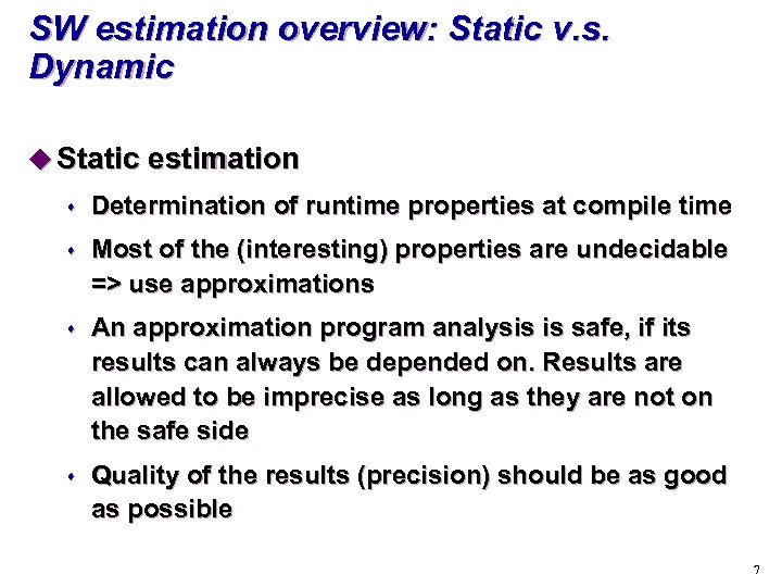
SW estimation overview: Static v. s. Dynamic u Static estimation s Determination of runtime properties at compile time s Most of the (interesting) properties are undecidable => use approximations s An approximation program analysis is safe, if its results can always be depended on. Results are allowed to be imprecise as long as they are not on the safe side s Quality of the results (precision) should be as good as possible 7

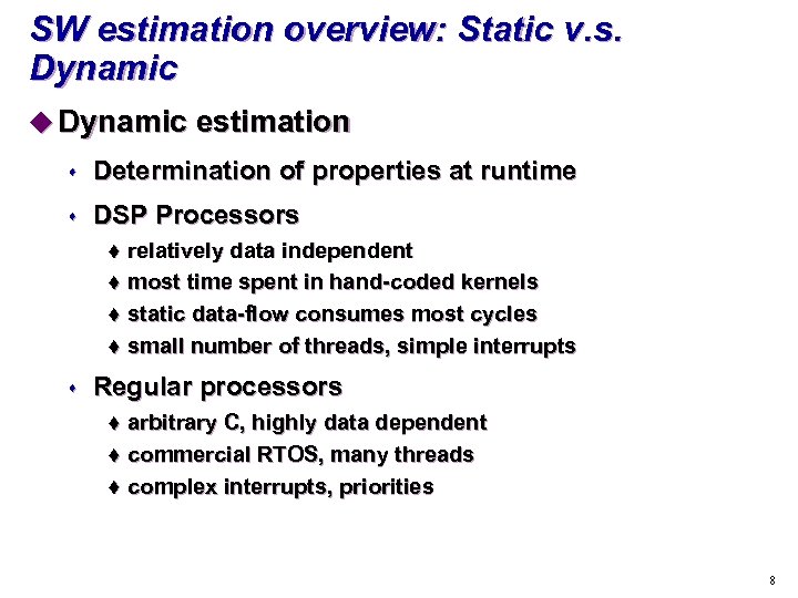
SW estimation overview: Static v. s. Dynamic u Dynamic estimation s Determination of properties at runtime s DSP Processors relatively data independent t most time spent in hand-coded kernels t static data-flow consumes most cycles t small number of threads, simple interrupts t s Regular processors arbitrary C, highly data dependent t commercial RTOS, many threads t complex interrupts, priorities t 8

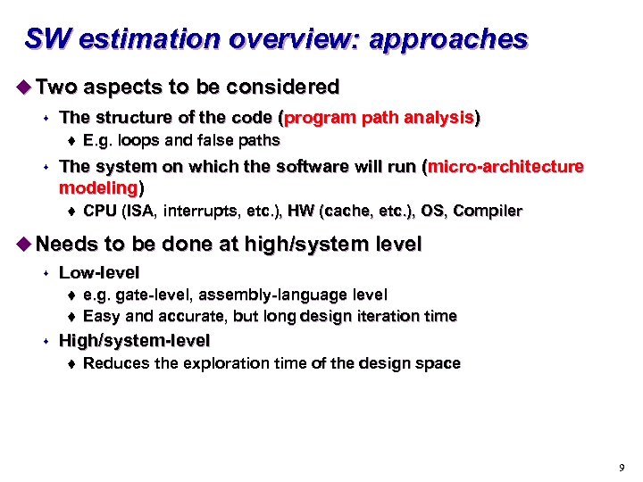
SW estimation overview: approaches u Two aspects to be considered s The structure of the code (program path analysis) t s E. g. loops and false paths The system on which the software will run (micro-architecture modeling) t CPU (ISA, interrupts, etc. ), HW (cache, etc. ), OS, Compiler u Needs to be done at high/system level s Low-level t t s e. g. gate-level, assembly-language level Easy and accurate, but long design iteration time High/system-level t Reduces the exploration time of the design space 9

Conventional system design flow Low-level performance estimation 10

System-level software model u Must be fast - whole system simulation u Processor model must be cheap s “what if” my processor did X s future processors not yet developed s evaluation of processor not currently used u Must be convenient to use s no need to compile with cross-compilers s debug on my desktop u Must be accurate enough for the purpose 11

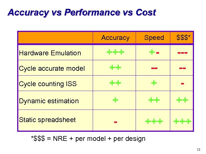
Accuracy vs Performance vs Cost Accuracy Speed $$$* Hardware Emulation +++ +- --- Cycle accurate model Cycle counting ISS ++ ++ -+ -- Dynamic estimation + ++ ++ Static spreadsheet - +++ *$$$ = NRE + per model + per design 12

Outline u. SW estimation overview u. Program path analysis u. Micro-architecture modeling u. Implementation examples: Cinderella u. SW estimation in VCC u. SW estimation in AI u. SW estimation in POLIS 13

Program path analysis u Basic blocks s A basic block is a program segment which is only entered at the first statement and only left at the last statement. s Example: function calls s The WCET (or BCET) of a basic block is determined u A program is divided into basic blocks s Program structure is represented on a directed program flow graph with basic blocks as nodes. s A longest / shortest path analysis on the program flow identify WCET / BCET 14

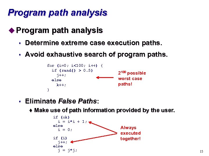
Program path analysis u Program path analysis s Determine extreme case execution paths. s Avoid exhaustive search of program paths. for (i=0; i<100; i++) { if (rand() > 0. 5) j++; else k++; } s 2100 possible worst case paths! Eliminate False Paths: t Make use of path information provided by the user. if (ok) i = i*i + 1; else i = 0; if (i) j++; else j = j*j; Always executed together! 15

Program path analysis u Path profile algorithm s Goal: Determines how many times each acyclic path in a routine executes s Method: identify sets of potential paths with states s Algorithms: Number final states from 0, 1, to n-1, where n is the number of potential paths in a routine; a final state represents the single path taken through a routine t Place instrumentation so that transitions need not occur at every conditional branch t Assign states so that transitions can be computed by a simple arithmetic operation t Transforms a control-flow graph containing loops or huge numbers of potential paths into an acyclic graph with a limited number of paths t 16

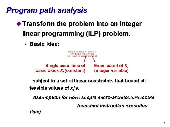
Program path analysis u Transform the problem into an integer linear programming (ILP) problem. s Basic idea: Single exec. time of basic block Bi (constant) Exec. count of Bi (integer variable) subject to a set of linear constraints that bound all feasible values of xi’s. Assumption for now: simple micro-architecture model (constant instruction execution time) 17

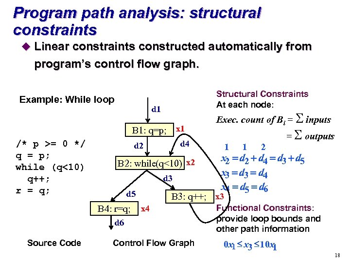
Program path analysis: structural constraints u Linear constraints constructed automatically from program’s control flow graph. Example: While loop Structural Constraints At each node: d 1 B 1: q=p; x 1 /* p >= 0 */ q = p; while (q<10) q++; r = q; d 4 d 2 B 2: while(q<10) x 2 d 3 d 5 B 4: r=q; 1 1 2 = S outputs x 2 = d 2 + d 4 = d 3 +d 5 x 3 = d 4 x 4 = d 5 = d 6 B 3: q++; x 3 x 4 d 6 Source Code Exec. count of Bi = S inputs Control Flow Graph Functional Constraints: provide loop bounds and other path information 0 x 1 £ x 3 £ 10 x 1 18

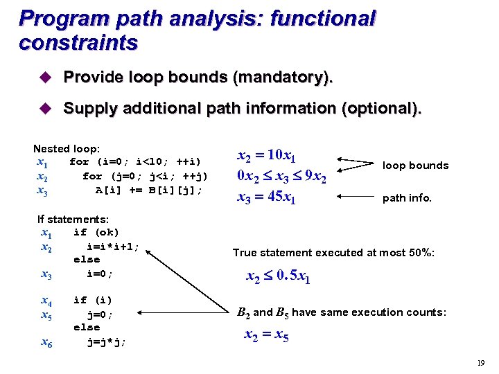
Program path analysis: functional constraints u Provide loop bounds (mandatory). u Supply additional path information (optional). Nested loop: x 1 for (i=0; i<10; ++i) x 2 for (j=0; j<i; ++j) x 3 A[i] += B[i][j]; If statements: x 1 if (ok) x 2 i=i*i+1; else x 3 i=0; x 4 x 5 x 6 if (i) j=0; else j=j*j; x 2 = 10 x 1 0 x 2 £ x 3 £ 9 x 2 x 3 = 45 x 1 loop bounds path info. True statement executed at most 50%: x 2 £ 0. 5 x 1 B 2 and B 5 have same execution counts: x 2 = x 5 19

Outline u. SW estimation overview u. Program path analysis u. Micro-architecture modeling u. Implementation examples: Cinderella u. SW estimation in VCC u. SW estimation in AI u. SW estimation in POLIS 20

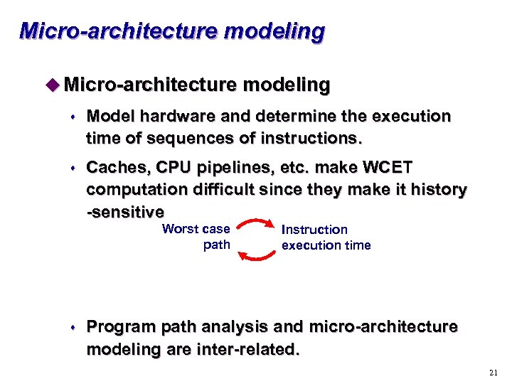
Micro-architecture modeling u Micro-architecture modeling s Model hardware and determine the execution time of sequences of instructions. s Caches, CPU pipelines, etc. make WCET computation difficult since they make it history -sensitive Worst case path s Instruction execution time Program path analysis and micro-architecture modeling are inter-related. 21

Micro-architecture modeling u Pipeline analysis s Determine each instruction’s worst case effective execution time by looking at its surrounding instructions within the same basic block. s Assume constant pipeline execution time for each basic block. u Cache analysis s Dominant factor. s Global analysis is required. s Must be done simultaneously with path analysis. 22

Micro-architecture modeling u Other architecture feature analysis s Data dependent instruction execution times t Typical for CISC architectures u s e. g. shift-and-add instructions Superscalar architectures 23

Micro-architecture modeling: pipeline features u Pipelines are hard to predict s Stalls depend on execution history and cache contents s Execution times depend on execution history u Worst case assumptions s Instruction execution cannot be overlapped s If a hazard cannot be safely excluded, it must be assumed to happen s For some architectures, hazard and non-hazard must be considered (interferences with instruction fetching and caches) u Branch prediction s Predict which branch to fetch based on t t Target address (backward branches in loops) History of that jump (branch history table) 24

Micro-architecture modeling: pipeline features u On average, branch prediction works well s Branch history correctly predicts most branches s Very low delays due to jump instructions u Branch prediction is hard to predict s Depends on execution history (branch history table) s Depends on pipeline: when does fetching occur? s Incorporates additional instruction fetches not along the execution path of the program (mispredictions) s Changes instruction cache quite significantly u Worst case scenarios s Instruction fetches occur along all possible execution paths s Prediction is wrong: re-fetch along other path 25

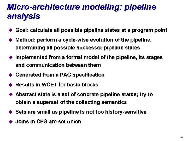
Micro-architecture modeling: pipeline analysis u Goal: calculate all possible pipeline states at a program point u Method: perform a cycle-wise evolution of the pipeline, determining all possible successor pipeline states u Implemented from a formal model of the pipeline, its stages and communication between them u Generated from a PAG specification u Results in WCET for basic blocks u Abstract state is a set of concrete pipeline states; try to obtain a superset of the collecting semantics u Sets are small as pipeline is not too history-sensitive u Joins in CFG are set union 26

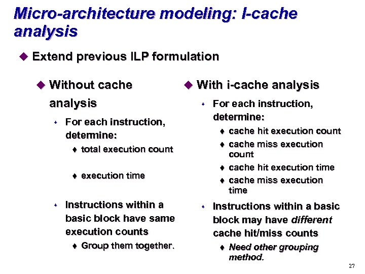
Micro-architecture modeling: I-cache analysis u Extend previous ILP formulation u Without cache analysis s s For each instruction, determine: t t s u With i-cache analysis t total execution count t execution time Instructions within a basic block have same execution counts Group them together. For each instruction, determine: t s cache hit execution count cache miss execution count cache hit execution time cache miss execution time Instructions within a basic block may have different cache hit/miss counts t Need other grouping method. 27

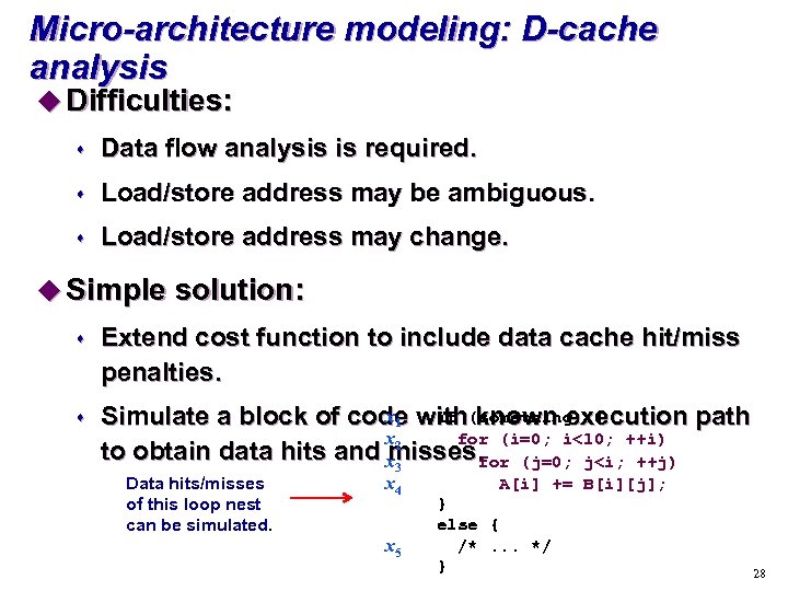
Micro-architecture modeling: D-cache analysis u Difficulties: s Data flow analysis is required. s Load/store address may be ambiguous. s Load/store address may change. u Simple solution: s Extend cost function to include data cache hit/miss penalties. s x 1 if known execution path Simulate a block of code with(something) { x for (i=0; i<10; ++i) to obtain data hits and x 2 misses. (j=0; j<i; ++j) for 3 Data hits/misses of this loop nest can be simulated. x 4 x 5 A[i] += B[i][j]; } else { /*. . . */ } 28

Outline u. SW estimation overview u. Program path analysis u. Micro-architecture modeling u. Implementation examples: Cinderella u. SW estimation in VCC u. SW estimation in AI u. SW estimation in POLIS 29

SW estimation in VCC Objectives u To be faster than co-simulation of the target processor (at least one order of magnitude) u To provide more flexible and easier to use bottleneck analysis than emulation (e. g. , who is causing the high cache miss rate? ) u To support fast design exploration (what-if analysis)after changes in the functionality and in the architecture u To support derivative design u To support well-designed legacy code (clear 30

SW estimation in VCC Approaches u. Various trade-offs between simplicity, compilation/simulation speed and precision u. Virtual Processor Model: it compiles C source to simplified “object code” used to back-annotate C source with execution cycle counts and memory accesses s Typically ISS uses object code, Cadence CC-ISS uses assembly code, commercial CC-ISS’s use object code u. CABA: C-Source Back Annotation and model calibration via Target Machine Instruction Set u. Instruction-Set Simulator: it uses target object code to: s either reconstruct annotated C source (Compiled-Code ISS) s or executed on an interpreted ISS 31

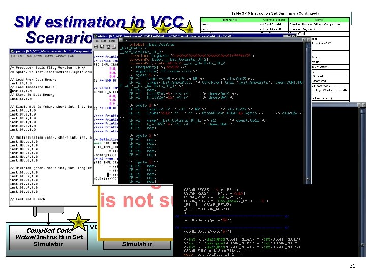
SW estimation in VCC Scenarios Target Processor Instruction Set White Box C Compiled Code Processor Model VCC Virtual Processor Instruction Set VCC Virtual Compiler Annotated White Box C Target Processor Compiler Target Assembly Code Host ASM 2 C Compiler Annotated White Box C . obj Host Compiler Compiled Code Virtual Instruction Set Simulator VCC Interpreted Compiled Code Instruction Set Simulator Co-simulation Instruction Set Simulator Target Processor 32

SW estimation in VCC Limitations u C (or assembler) library routine estimation (e. g. trigonometric functions): the delay should be part of the library model u Import of arbitrary (especially processor or RTOS-dependent) legacy code s Code must adhere to the simulator interface including embedded system calls (RTOS): the conversion is not the aim of software estimation 33

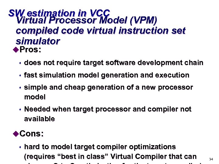
SW estimation in VCC Virtual Processor Model (VPM) compiled code virtual instruction set simulator u. Pros: s does not require target software development chain s fast simulation model generation and execution s simple and cheap generation of a new processor model s Needed when target processor and compiler not available u. Cons: s hard to model target compiler optimizations (requires “best in class” Virtual Compiler that can 34

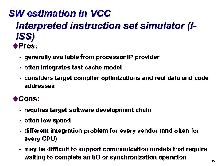
SW estimation in VCC Interpreted instruction set simulator (IISS) u. Pros: s generally available from processor IP provider s often integrates fast cache model s considers target compiler optimizations and real data and code addresses u. Cons: s requires target software development chain s often low speed s different integration problem for every vendor (and often for every CPU) s may be difficult to support communication models that require waiting to complete an I/O or synchronization operation 35

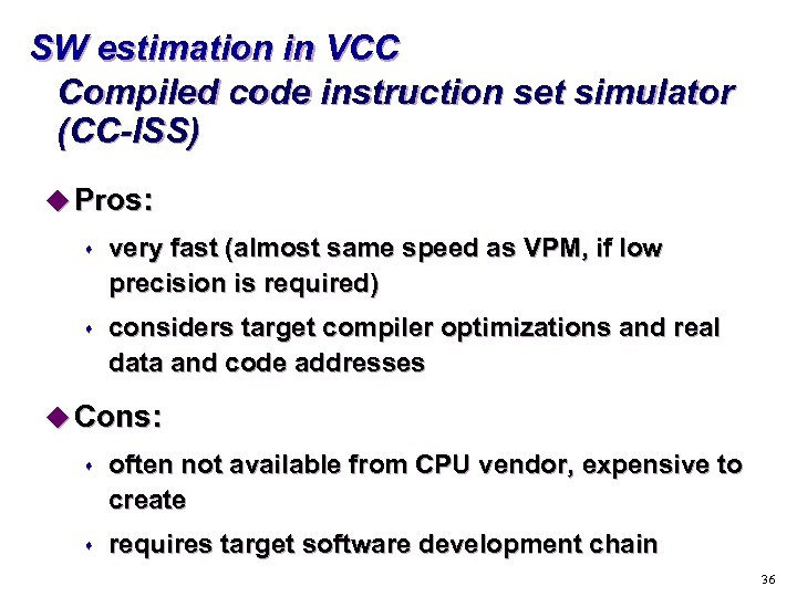
SW estimation in VCC Compiled code instruction set simulator (CC-ISS) u Pros: s very fast (almost same speed as VPM, if low precision is required) s considers target compiler optimizations and real data and code addresses u Cons: s often not available from CPU vendor, expensive to create s requires target software development chain 36

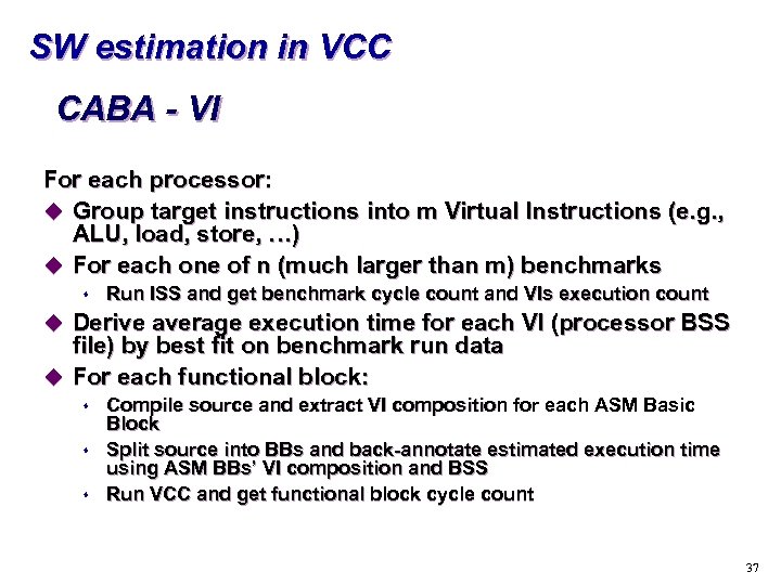
SW estimation in VCC CABA - VI For each processor: u Group target instructions into m Virtual Instructions (e. g. , ALU, load, store, …) u For each one of n (much larger than m) benchmarks s Run ISS and get benchmark cycle count and VIs execution count u Derive average execution time for each VI (processor BSS file) by best fit on benchmark run data u For each functional block: s s s Compile source and extract VI composition for each ASM Basic Block Split source into BBs and back-annotate estimated execution time using ASM BBs’ VI composition and BSS Run VCC and get functional block cycle count 37

SW estimation in VCC CABA - VI u CABA-VI: uses a calibration-like procedure to obtain average execution timing for each target instruction (or instruction class – Virtual Instruction (VI)). Unlike the similar VPM technique, the VI’s are target-dependent. The resulted BSS is used to generate the performance annotations (delay, power, bus traffic) and its accuracy is not limited to the calibration codes. u In both cases, part of the CCISS infrastructure is reused to: s s s parse the assembler, identify the basic blocks, identify and remove the cross-reference tags, handle embedded waits and other constructs, generate code for bus traffic. 38

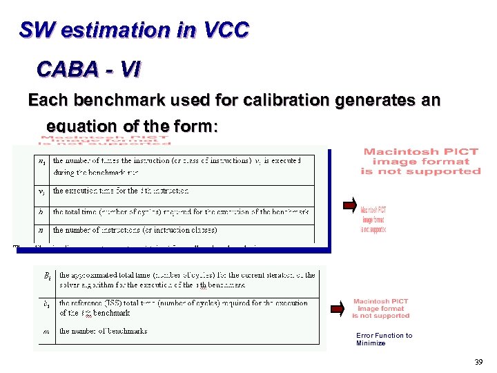
SW estimation in VCC CABA - VI Each benchmark used for calibration generates an equation of the form: Error Function to Minimize 39

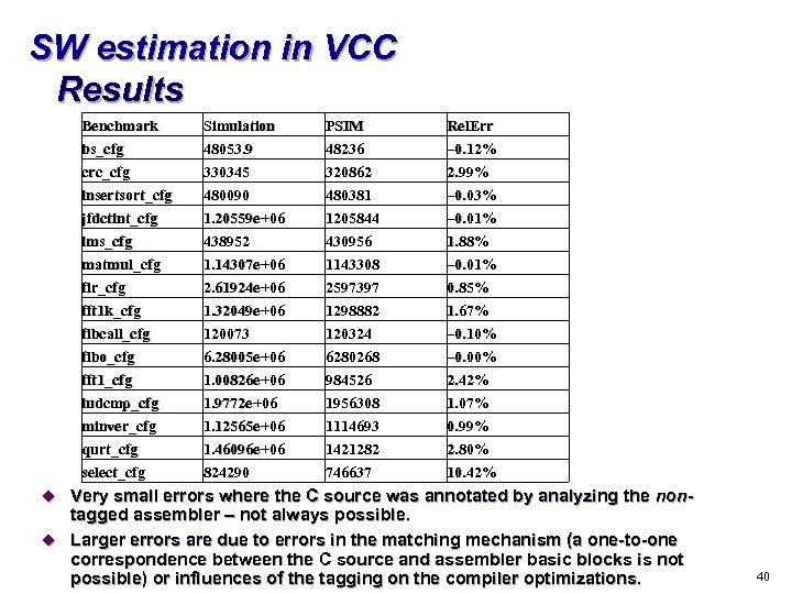
SW estimation in VCC Results Benchmark bs_cfg crc_cfg insertsort_cfg jfdctint_cfg lms_cfg Simulation 48053. 9 330345 480090 1. 20559 e+06 438952 PSIM 48236 320862 480381 1205844 430956 Rel. Err – 0. 12% 2. 99% – 0. 03% – 0. 01% 1. 88% matmul_cfg fir_cfg fft 1 k_cfg fibcall_cfg fibo_cfg fft 1_cfg ludcmp_cfg minver_cfg qurt_cfg select_cfg 1. 14307 e+06 2. 61924 e+06 1. 32049 e+06 120073 6. 28005 e+06 1. 00826 e+06 1. 9772 e+06 1. 12565 e+06 1. 46096 e+06 824290 1143308 2597397 1298882 120324 6280268 984526 1956308 1114693 1421282 746637 – 0. 01% 0. 85% 1. 67% – 0. 10% – 0. 00% 2. 42% 1. 07% 0. 99% 2. 80% 10. 42% u Very small errors where the C source was annotated by analyzing the non- tagged assembler – not always possible. u Larger errors are due to errors in the matching mechanism (a one-to-one correspondence between the C source and assembler basic blocks is not possible) or influences of the tagging on the compiler optimizations. 40

SW estimation in VCC Conclusions u VPM-C s s s s s Features a high accuracy when simulating the code it was tuned for. The BSS file generation can be automated In case of limited code coverage during the BSS generation phase, it might feature unpredictable accuracy variations when the code or input data changes. The code coverage depends also on the data set used as input to generate the model. Assumes a perfect cache. Requires cycle accurate ISS and target compiler (only by the modeler not by the user of the model) Good for achieving accurate simulations for data dominated flows, whose control flow remains pretty much unchanged with data variations (e. g. , MPEG decoding) Development time for a new BSS ranges from 1 day to 1 week. Fine tuning the BSS to improve the accuracy may go up to 1 month, mostly due to extensive simulations Good if not developing extremely time-critical software (e. g. Interrupt Service Routines), or when the precision of SWE is sufficient for the task at hand (e. g. , not for final validation after partial integration on an ECU) 41

SW estimation in VCC Conclusions u CABA s Fast simulation, comparable with VPM. s Good to very good accuracy, since the measurements are based on the real assembler and target architecture effects. s Good stability with respect to code or execution flow changes s The production target compiler is needed (both modeler and user) s About 1 man-month for building a CABA-VI infrastructure, with one processor model. s From 2 weeks to 2 months to integrate a new processor – depending upon the simulation time required for the calibration s Combines the fast simulation, that characterizes the VPMbased techniques, with the high accuracy of the object code analysis techniques, such as CCISS and ISS integration. s Although too few experiments were conducted to know how well it suits various kinds of targets and what is its accuracy and stability to input data and control flow variations, they 42