Software Analysis Status R Sawada MEG Review

Software & Analysis Status R. Sawada MEG Review Meeting PSI, 18 July 2007

Outline • • Software framework (Just for reminding) Online Simulation Analysis • • • Reconstruction Physics analysis Computing Man power Summary Abbreviations XEC : Liquid xenon calorimeter TC : Timing counter TICP : TC Phi measuring counter (Bars) TICZ : TC Z measuring counter (Fibers) DCH : Drift chambers RD : Radiative decay WF : Waveform B. R. : Branching ratio AIF : Annihilation in flight MC : Monte-Carlo simulation 2

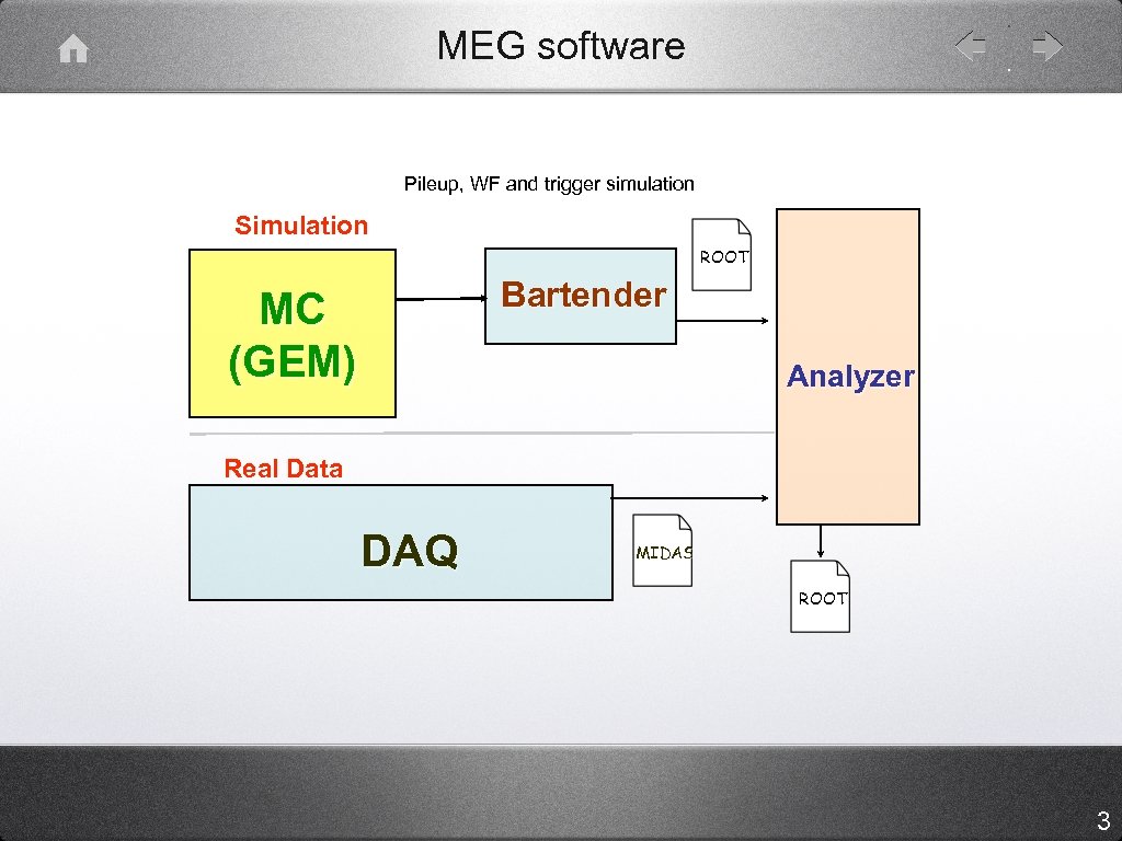MEG software Pileup, WF and trigger simulation Simulation ROOT Bartender MC (GEM) Analyzer Real Data DAQ MIDAS ROOT 3

Status of software group • Sub groups have regular internet meetings • • New module for “global” analysis was added • • Event pre-selection, sub-detecter inter-calibration, parameters for physics analysis Developers of analyzer is increasing, especially students • • DCH, TC, XEC, data reduction and physics working group Thanks to ROME(automatic code generation system developed in MEG), new comers start development smoothly Quality control of software is getting important • • Standard test procedure of software was introduced. Everybody makes the check of software with a standard data set, with identical configuration files at every time after commits 4

Online (data reduction)

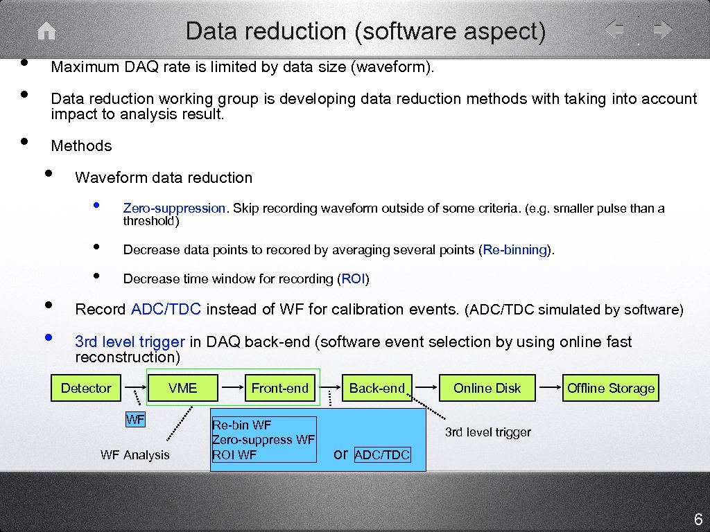Data reduction (software aspect) • • • Maximum DAQ rate is limited by data size (waveform). Data reduction working group is developing data reduction methods with taking into account impact to analysis result. Methods • Waveform data reduction • Zero-suppression. Skip recording waveform outside of some criteria. (e. g. smaller pulse than a threshold) • • Decrease data points to recored by averaging several points (Re-binning). Decrease time window for recording (ROI) Record ADC/TDC instead of WF for calibration events. (ADC/TDC simulated by software) 3 rd level trigger in DAQ back-end (software event selection by using online fast reconstruction) Detector VME WF WF Analysis Front-end Re-bin WF Zero-suppress WF ROI WF Back-end Online Disk Offline Storage 3 rd level trigger or ADC/TDC 6

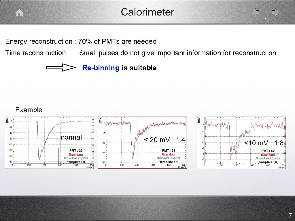Calorimeter Energy reconstruction : 70% of PMTs are needed Time reconstruction : Small pulses do not give important information for reconstruction Re-binning is suitable Example normal < 20 m. V, 1: 4 <10 m. V, 1: 8 7

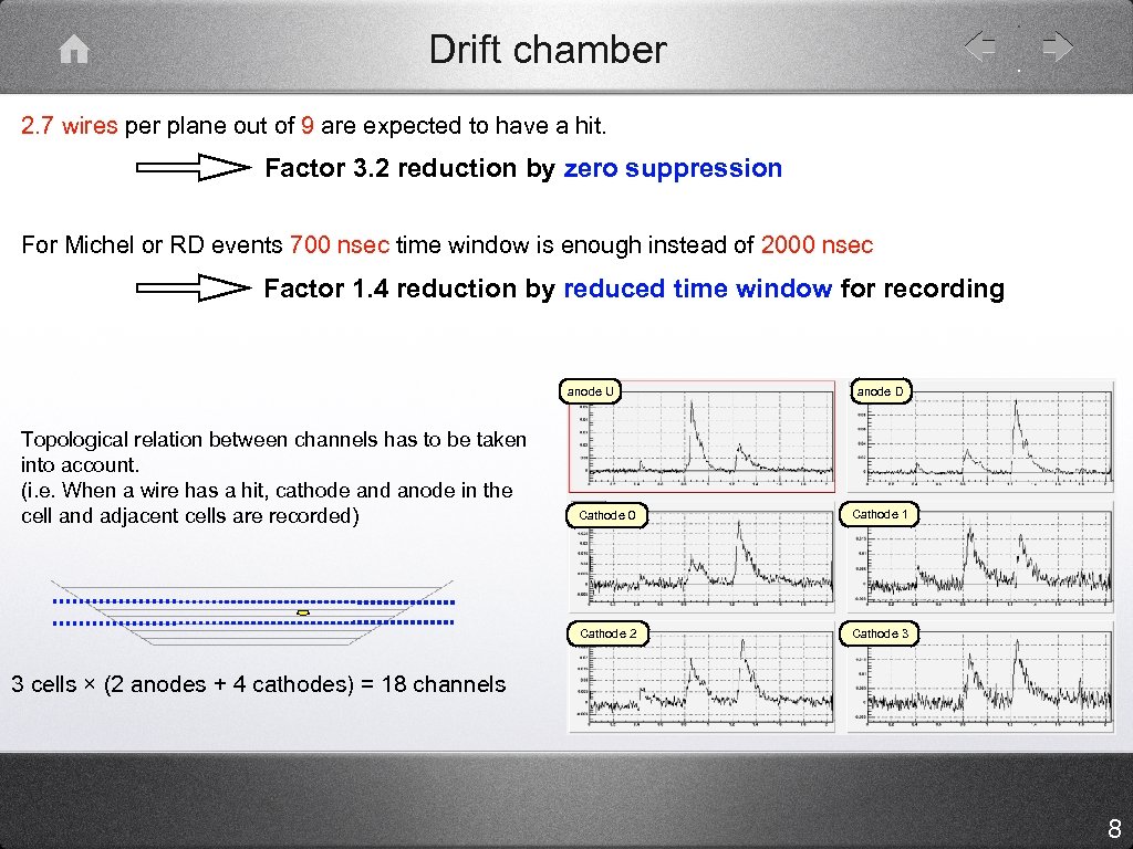Drift chamber 2. 7 wires per plane out of 9 are expected to have a hit. Factor 3. 2 reduction by zero suppression For Michel or RD events 700 nsec time window is enough instead of 2000 nsec Factor 1. 4 reduction by reduced time window for recording anode U Topological relation between channels has to be taken into account. (i. e. When a wire has a hit, cathode and anode in the cell and adjacent cells are recorded) anode D Cathode 0 Cathode 1 Cathode 2 Cathode 3 3 cells × (2 anodes + 4 cathodes) = 18 channels 8

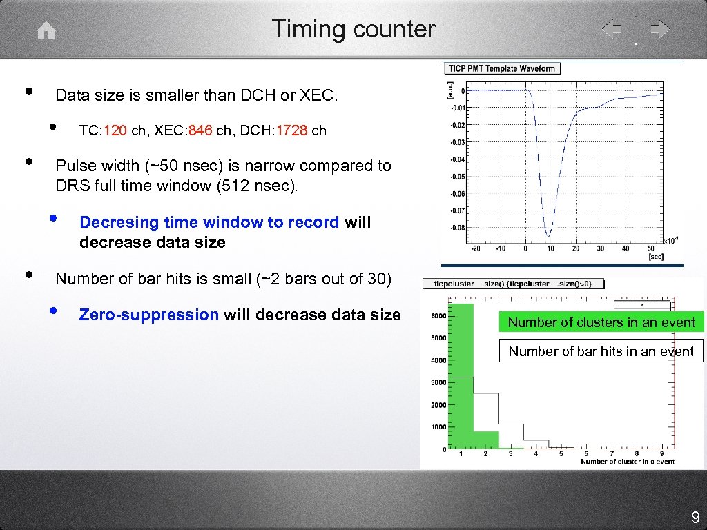Timing counter • Data size is smaller than DCH or XEC. • • Pulse width (~50 nsec) is narrow compared to DRS full time window (512 nsec). • • TC: 120 ch, XEC: 846 ch, DCH: 1728 ch Decresing time window to record will decrease data size Number of bar hits is small (~2 bars out of 30) • Zero-suppression will decrease data size Number of clusters in an event Number of bar hits in an event 9

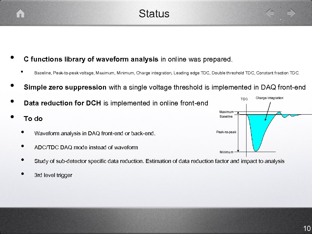Status • C functions library of waveform analysis in online was prepared. • • Baseline, Peak-to-peak voltage, Maximum, Minimum, Charge integration, Leading edge TDC, Double threshold TDC, Constant fraction TDC. Simple zero suppression with a single voltage threshold is implemented in DAQ front-end TDC Data reduction for DCH is implemented in online front-end To do • • Waveform analysis in DAQ front-end or back-end. ADC/TDC DAQ mode instead of waveform Charge integration Maximum Baseline Peak-to-peak Minimum Study of sub-detector specific data reduction. Estimation of data reduction factor and impact to analysis 3 rd level trigger 10

Simulation

MC(GEM) updates • Event generation • • AIF probability enhanced mode. (Preliminary) Radiative decay • • • More flexible configuration keys to specify generation condition. (energy cuts and opening angle) Calculation of phase volume (branching ratio) of specified kinematic range Geometry updates • • • Geometry for this year’s setup Details (target, honeycomb panel of calorimeter, alpha source. . ) Better simulation of drift electron in chambers. (diffusion included) 12

MC(Bartender) updates • • Reorganization of MC hit structures of each modules (DCH, TIC[P/Z], XEC) to be easier to compare with reconstruction. Waveform simulation updates. • • • DCH : Response function from X-ray source data XEC : Precise TTS simulation, Attenuators in DRS, Clipping before splitter. Several performance improvements for collecting data in signal region. • • 1. 2 sec/event/CPU for prompt background 1. 3 sec/event/CPU for accidental background 13

Analysis Figures and numbers will be shown. These are all preliminary, just for status report. All studies are using MC data. (Pure signal, or assuming 3 E 7 muon stopping rate)

Drift chamber

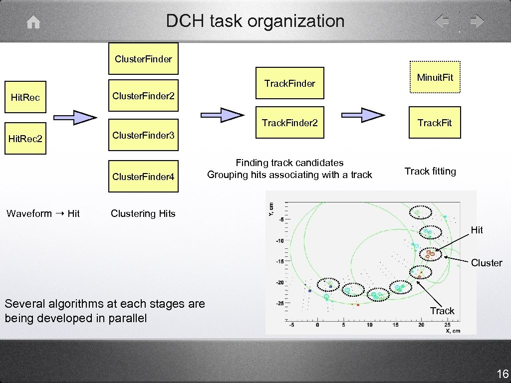DCH task organization Cluster. Finder Track. Finder Hit. Rec Cluster. Finder 2 Track. Finder 2 Hit. Rec 2 Track. Fit Cluster. Finder 3 Cluster. Finder 4 Waveform ➝ Hit Minuit. Fit Finding track candidates Grouping hits associating with a track Track fitting Clustering Hits Hit Cluster Several algorithms at each stages are being developed in parallel Track 16

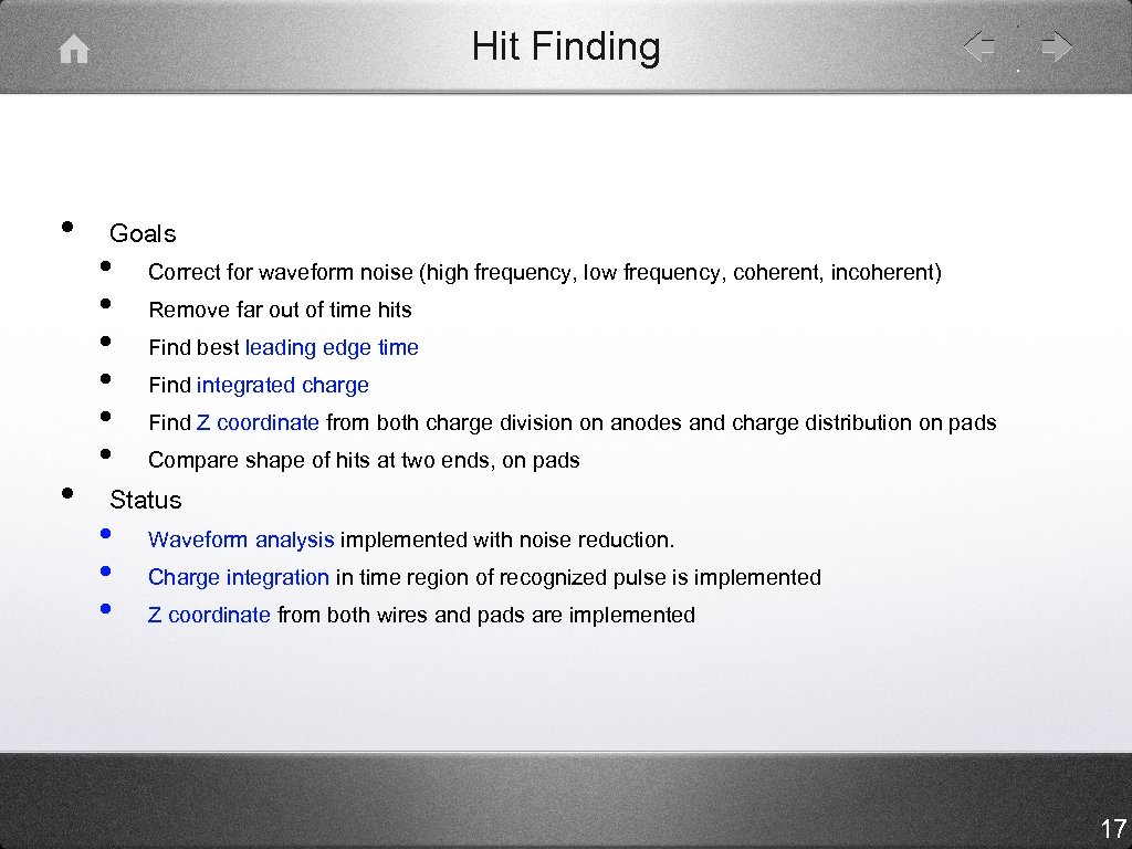Hit Finding • • Goals • • • Correct for waveform noise (high frequency, low frequency, coherent, incoherent) Remove far out of time hits Find best leading edge time Find integrated charge Find Z coordinate from both charge division on anodes and charge distribution on pads Compare shape of hits at two ends, on pads Status • • • Waveform analysis implemented with noise reduction. Charge integration in time region of recognized pulse is implemented Z coordinate from both wires and pads are implemented 17

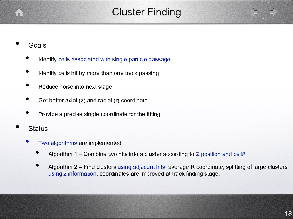Cluster Finding • Goals • • • Identify cells associated with single particle passage Identify cells hit by more than one track passing Reduce noise into next stage Get better axial (z) and radial (r) coordinate Provide a precise single coordinate for the fitting Status • Two algorithms are implemented • • Algorithm 1 – Combine two hits into a cluster according to Z position and cell#. Algorithm 2 – Find clusters using adjacent hits, average R coordinate, splitting of large clusters using z information. coordinates are improved at track finding stage. 18

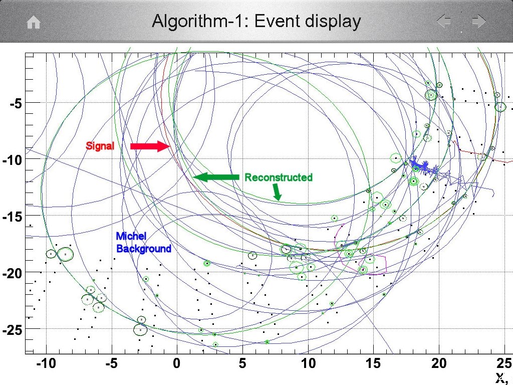
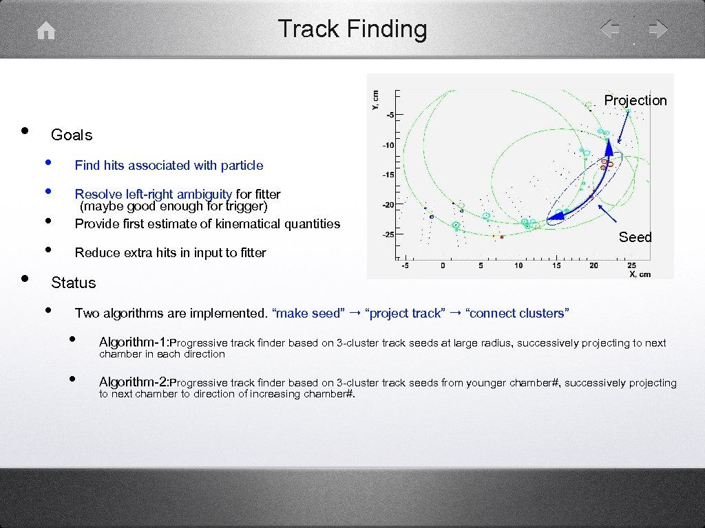Track Finding Projection • Goals • • • Find hits associated with particle Resolve left-right ambiguity for fitter (maybe good enough for trigger) Provide first estimate of kinematical quantities Reduce extra hits in input to fitter Seed Status • Two algorithms are implemented. “make seed” ➝ “project track” ➝ “connect clusters” • Algorithm-1: Progressive track finder based on 3 -cluster track seeds at large radius, successively projecting to next • Algorithm-2: Progressive track finder based on 3 -cluster track seeds from younger chamber#, successively projecting chamber in each direction to next chamber to direction of increasing chamber#.

Algorithm-1: Event display 20

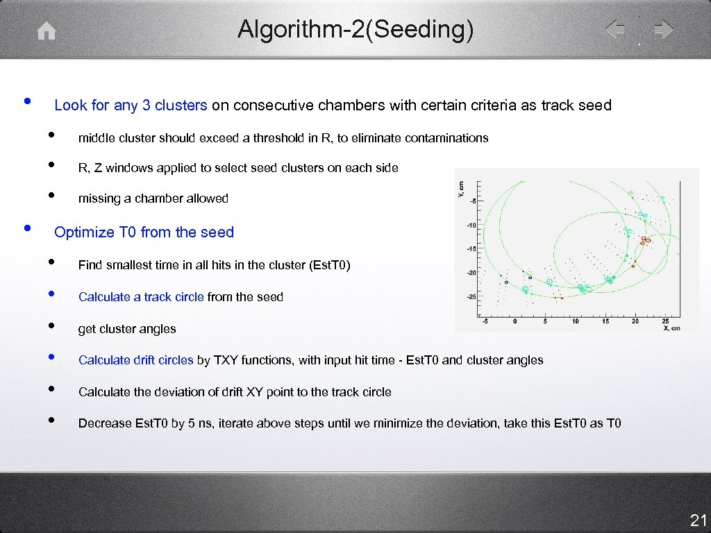Algorithm-2(Seeding) • Look for any 3 clusters on consecutive chambers with certain criteria as track seed • • middle cluster should exceed a threshold in R, to eliminate contaminations R, Z windows applied to select seed clusters on each side missing a chamber allowed Optimize T 0 from the seed • • • Find smallest time in all hits in the cluster (Est. T 0) Calculate a track circle from the seed get cluster angles Calculate drift circles by TXY functions, with input hit time - Est. T 0 and cluster angles Calculate the deviation of drift XY point to the track circle Decrease Est. T 0 by 5 ns, iterate above steps until we minimize the deviation, take this Est. T 0 as T 0 21

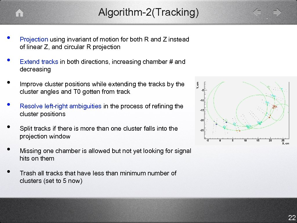Algorithm-2(Tracking) • • Projection using invariant of motion for both R and Z instead of linear Z, and circular R projection Extend tracks in both directions, increasing chamber # and decreasing Improve cluster positions while extending the tracks by the cluster angles and T 0 gotten from track Resolve left-right ambiguities in the process of refining the cluster positions Split tracks if there is more than one cluster falls into the projection window Missing one chamber is allowed but not yet looking for signal hits on them Trash all tracks that have less than minimum number of clusters (set to 5 now) 22

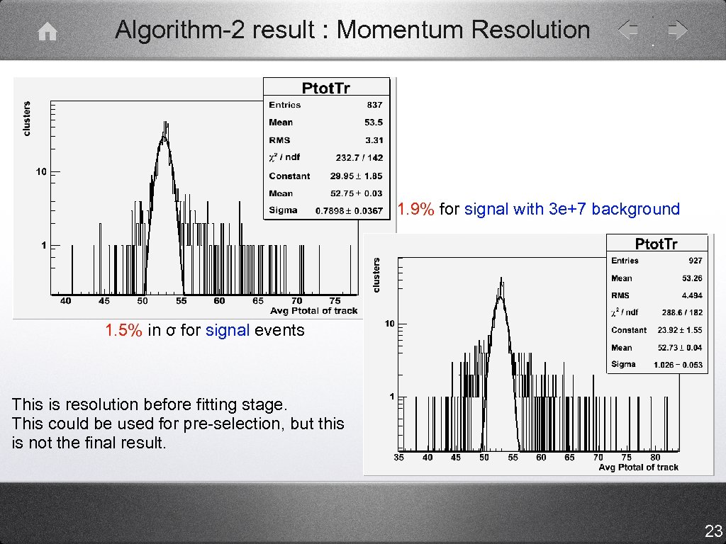Algorithm-2 result : Momentum Resolution 1. 9% for signal with 3 e+7 background 1. 5% in σ for signal events This is resolution before fitting stage. This could be used for pre-selection, but this is not the final result. 23

Track Fitting • Goals • • Determine quality of fit, identify poorly fit tracks Determine precision of measurements Kalman filter exists • • Find best kinematical quantities Finds kinematical quantities and state vector of tracks at different points in trajectory Alternative fitter using MINUIT • • Make use of integration of equation of motion in vacuum. This is written in Fortran code. Need to be implemented in analyzer. 24

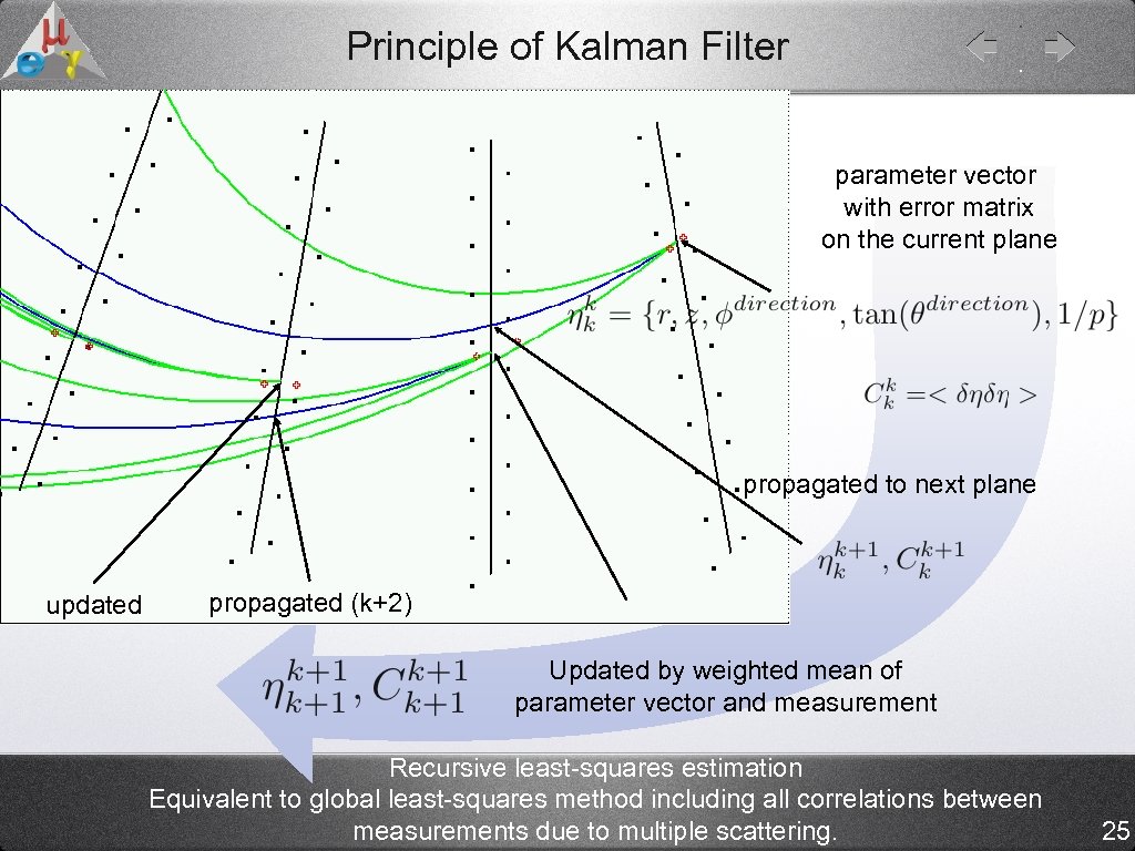Principle of Kalman Filter parameter vector with error matrix on the current plane propagated to next plane updated propagated (k+2) Updated by weighted mean of parameter vector and measurement Recursive least-squares estimation Equivalent to global least-squares method including all correlations between measurements due to multiple scattering. 25

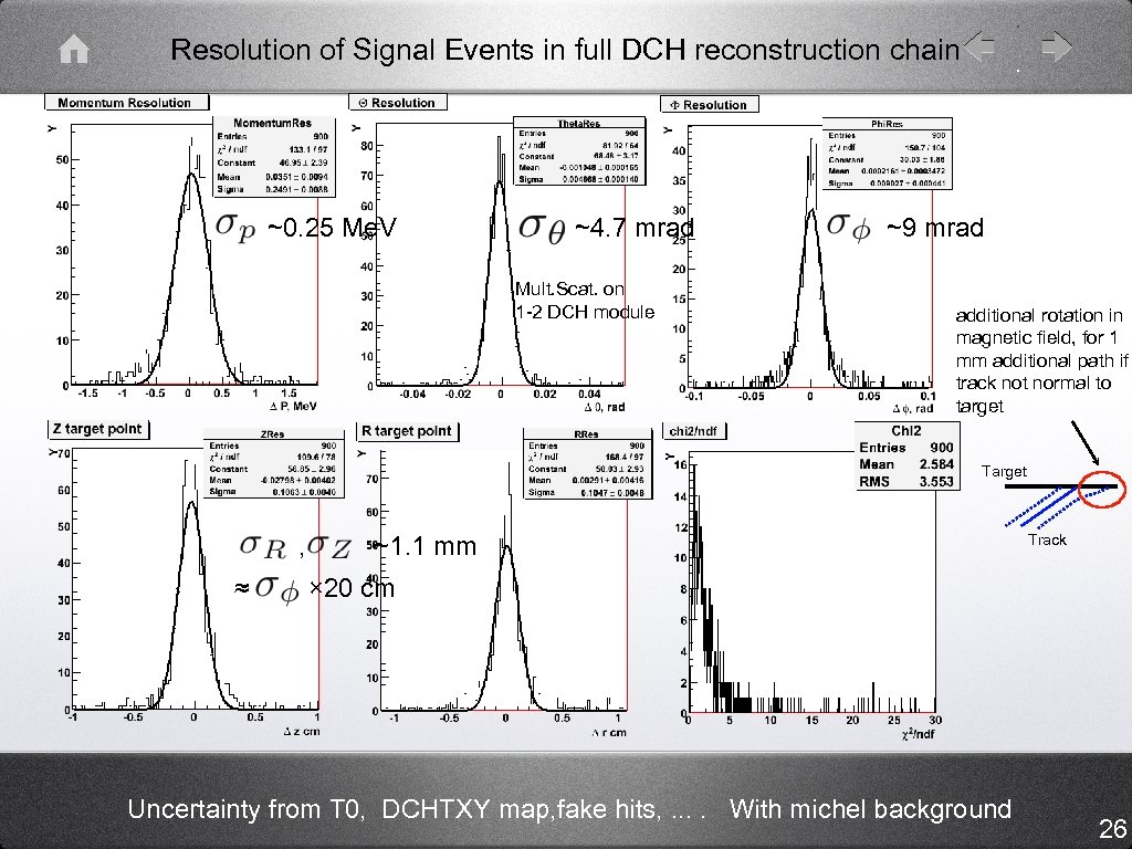Resolution of Signal Events in full DCH reconstruction chain ~0. 25 Me. V ~4. 7 mrad Mult. Scat. on 1 -2 DCH module ~9 mrad additional rotation in magnetic field, for 1 mm additional path if track not normal to target Target , ≈ ~1. 1 mm Track × 20 cm Uncertainty from T 0, DCHTXY map, fake hits, . . With michel background 26

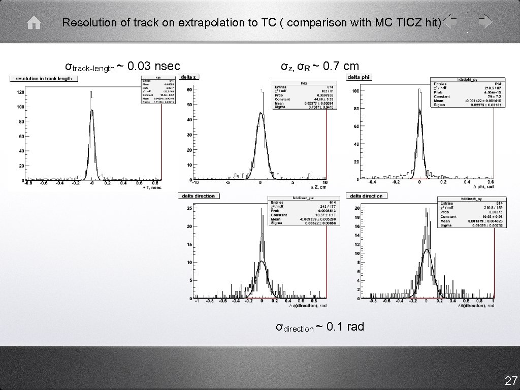Resolution of track on extrapolation to TC ( comparison with MC TICZ hit) σtrack-length ~ 0. 03 nsec σz, σR ~ 0. 7 cm σdirection ~ 0. 1 rad 27

Timing counter

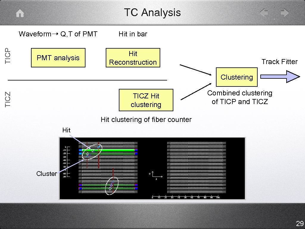TC Analysis TICP Waveform➝ Q, T of PMT Hit in bar PMT analysis Hit Reconstruction Track Fitter TICZ Clustering TICZ Hit clustering Combined clustering of TICP and TICZ Hit clustering of fiber counter Hit Cluster 29

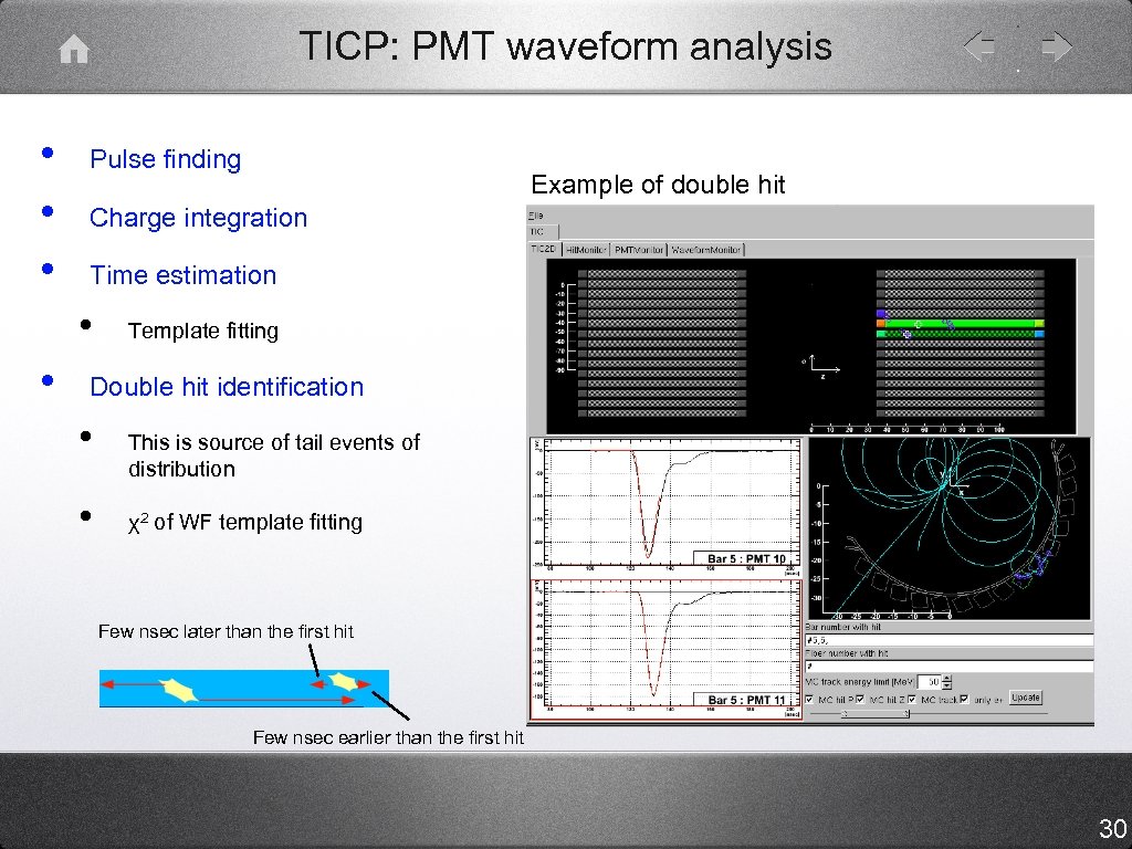TICP: PMT waveform analysis • • • Pulse finding Charge integration Time estimation • • Example of double hit Template fitting Double hit identification • • This is source of tail events of distribution χ2 of WF template fitting Few nsec later than the first hit Few nsec earlier than the first hit 30

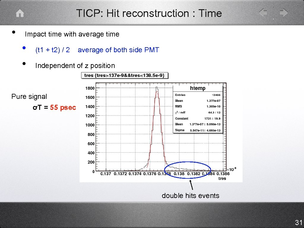TICP: Hit reconstruction : Time • Impact time with average time • • (t 1 + t 2) / 2 average of both side PMT Independent of z position Pure signal σT = 55 psec double hits events 31

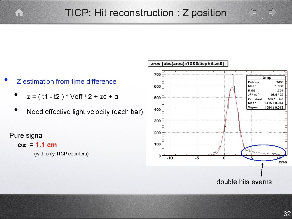TICP: Hit reconstruction : Z position • Z estimation from time difference • • z = ( t 1 - t 2 ) * Veff / 2 + zc + α Need effective light velocity (each bar) Pure signal σz = 1. 1 cm (with only TICP counters) double hits events 32

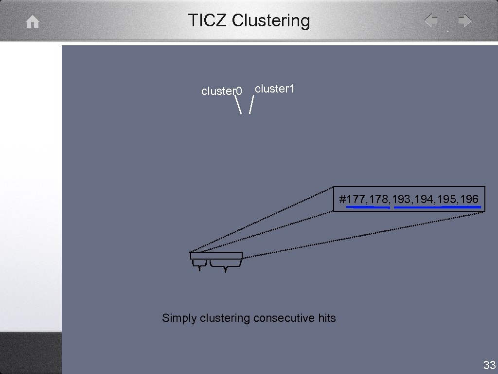TICZ Clustering cluster 0 cluster 1 #177, 178, 193, 194, 195, 196 Simply clustering consecutive hits 33

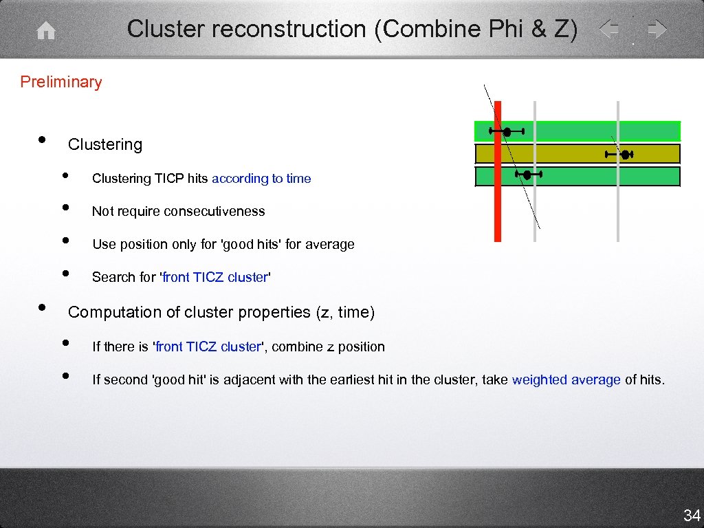Cluster reconstruction (Combine Phi & Z) Preliminary • Clustering • • • Clustering TICP hits according to time Not require consecutiveness Use position only for 'good hits' for average Search for 'front TICZ cluster' Computation of cluster properties (z, time) • • If there is 'front TICZ cluster', combine z position If second 'good hit' is adjacent with the earliest hit in the cluster, take weighted average of hits. 34

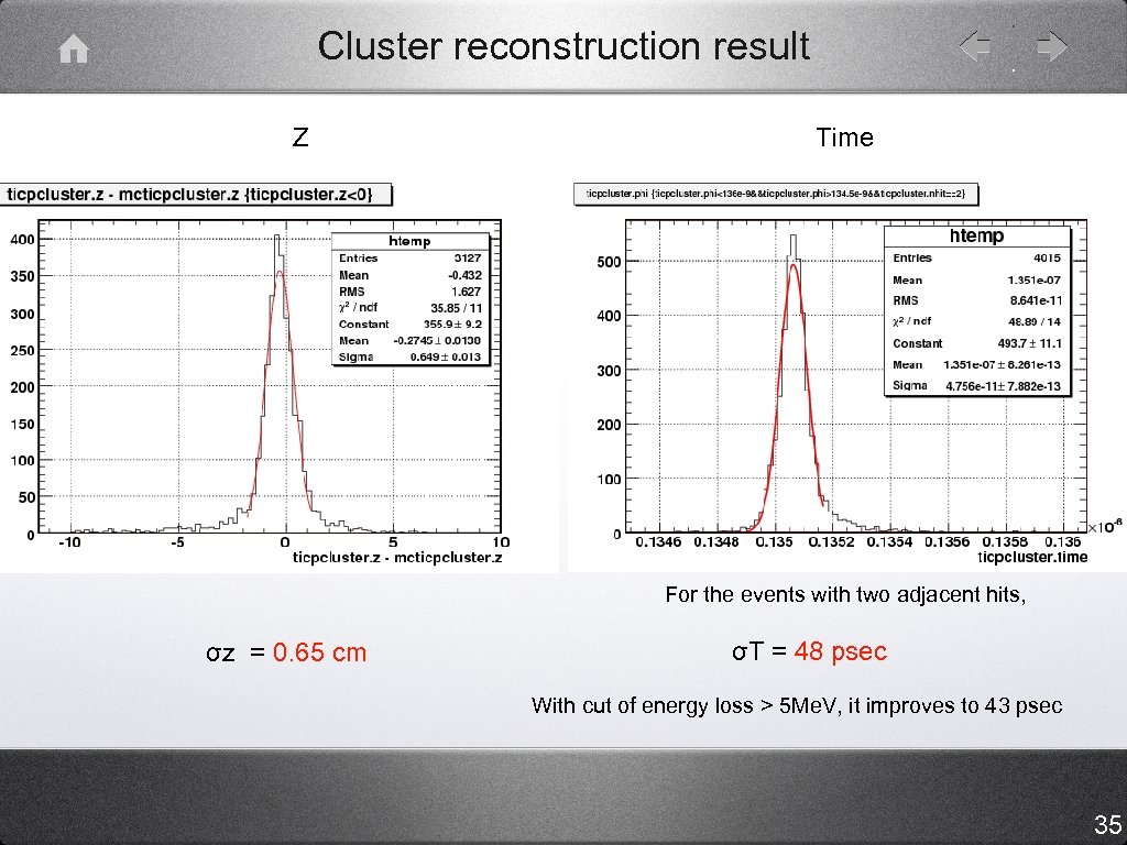Cluster reconstruction result Z Time For the events with two adjacent hits, σz = 0. 65 cm σT = 48 psec With cut of energy loss > 5 Me. V, it improves to 43 psec 35

Calorimeter

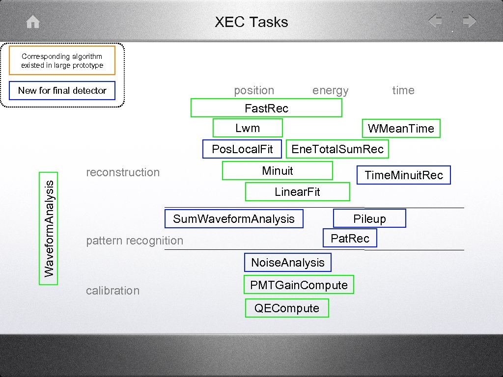XEC Tasks Corresponding algorithm existed in large prototype position New for final detector energy time Fast. Rec Lwm WMean. Time Pos. Local. Fit Minuit reconstruction Waveform. Analysis Ene. Total. Sum. Rec Time. Minuit. Rec Linear. Fit Pileup Sum. Waveform. Analysis Pat. Rec pattern recognition Noise. Analysis calibration PMTGain. Compute QECompute

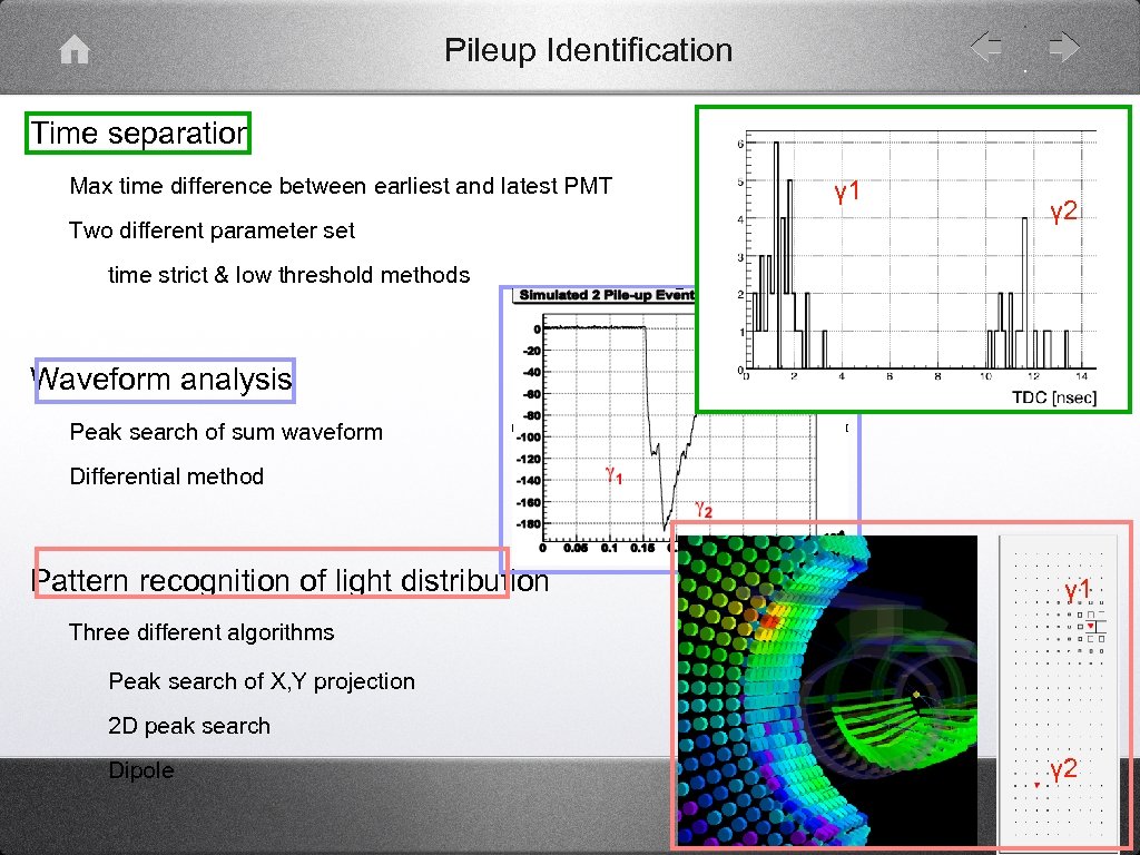Pileup Identification Time separation Max time difference between earliest and latest PMT Two different parameter set γ 1 γ 2 time strict & low threshold methods Waveform analysis Peak search of sum waveform Differential method Pattern recognition of light distribution γ 1 Three different algorithms Peak search of X, Y projection 2 D peak search Dipole γ 2

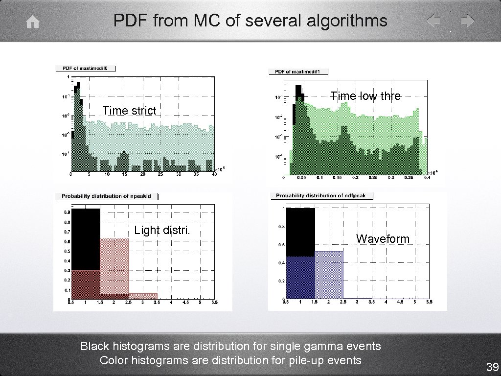PDF from MC of several algorithms Time low thre Time strict Light distri. Waveform Black histograms are distribution for single gamma events Color histograms are distribution for pile-up events 39

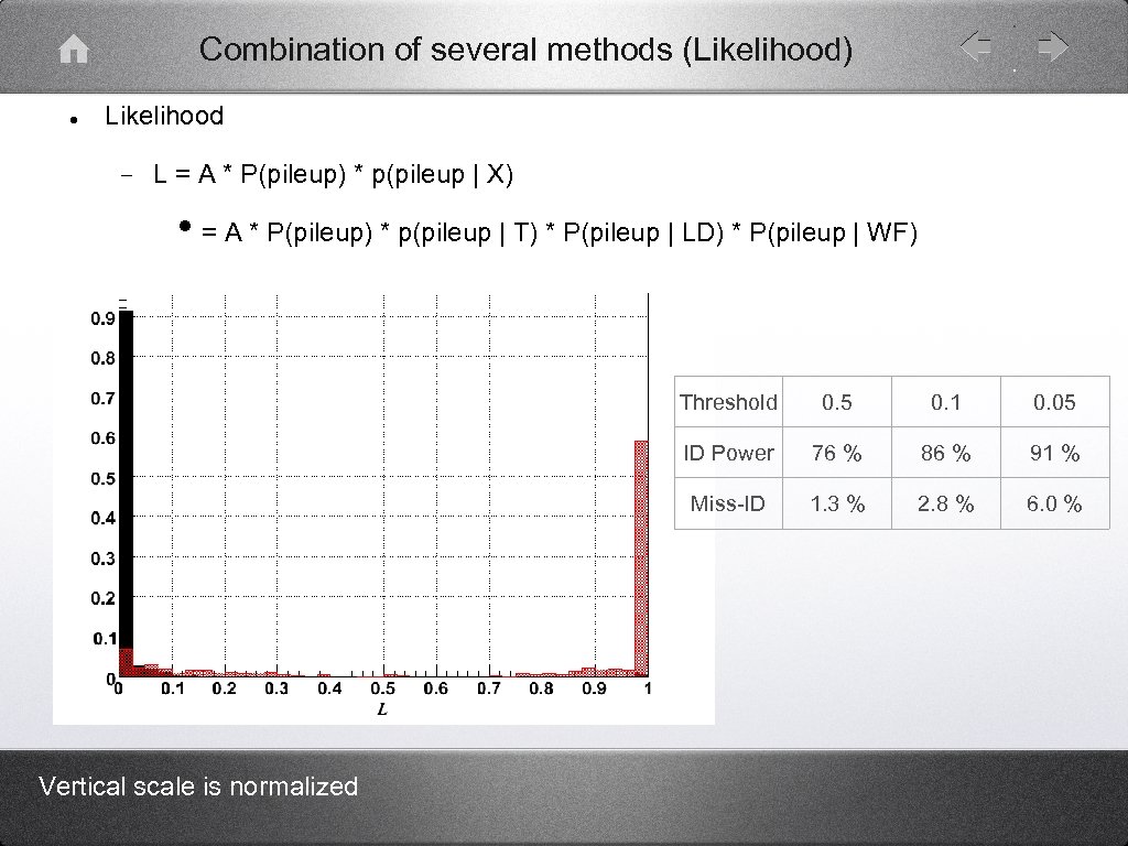Combination of several methods (Likelihood) l Likelihood − L = A * P(pileup) * p(pileup | X) • = A * P(pileup) * p(pileup | T) * P(pileup | LD) * P(pileup | WF) Threshold 0. 1 0. 05 ID Power 76 % 86 % 91 % Miss-ID Vertical scale is normalized 0. 5 1. 3 % 2. 8 % 6. 0 %

Physics

Outline • Maximum likelihood 1. 2. • • How to build likelihood function? Sensitivity study using PDF from known detector performance. (using different data set from 1. ) Blind μ→eγ analysis Possible analysis procedure 42

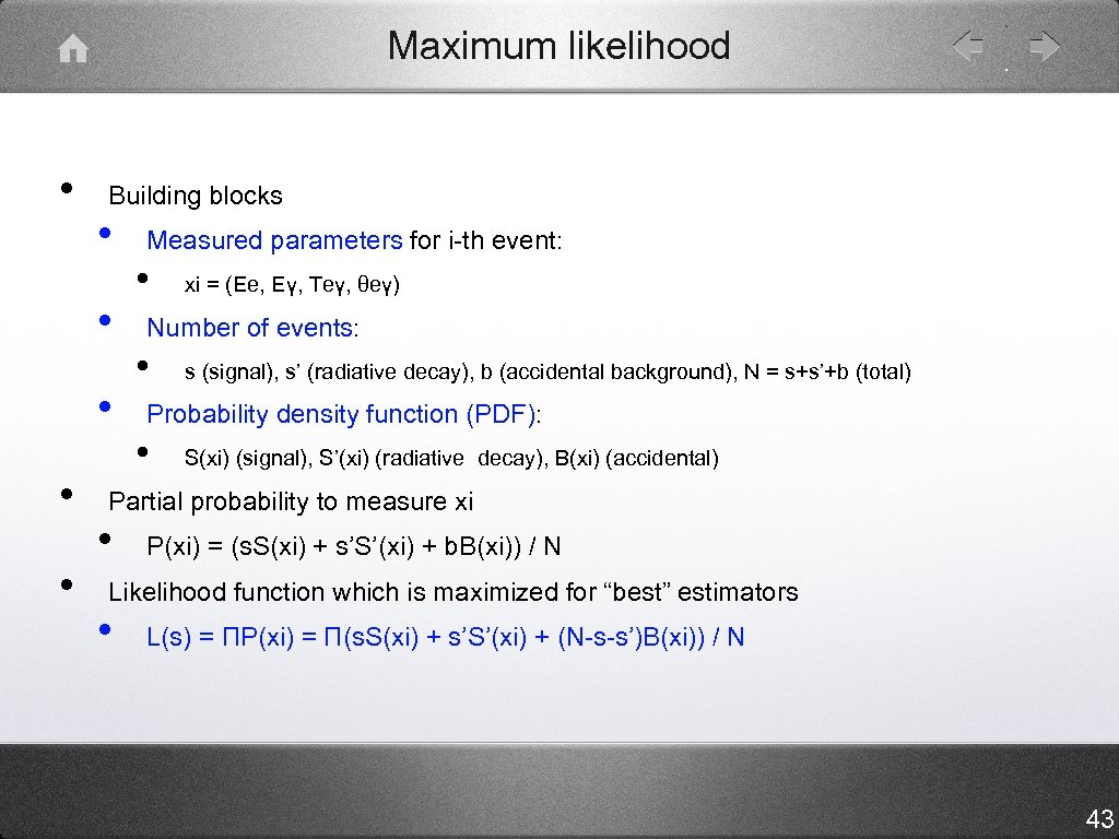Maximum likelihood • Building blocks • • • Measured parameters for i-th event: • xi = (Ee, Eγ, Teγ, θeγ) Number of events: • s (signal), s’ (radiative decay), b (accidental background), N = s+s’+b (total) Probability density function (PDF): • S(xi) (signal), S’(xi) (radiative decay), B(xi) (accidental) Partial probability to measure xi • P(xi) = (s. S(xi) + s’S’(xi) + b. B(xi)) / N Likelihood function which is maximized for “best” estimators • L(s) = ΠP(xi) = Π(s. S(xi) + s’S’(xi) + (N-s-s’)B(xi)) / N 43

How to build PDF ?

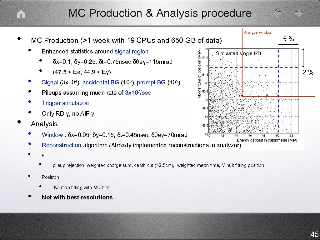MC Production & Analysis procedure • • Analysis window MC Production (>1 week with 19 CPUs and 650 GB of data) • • • Enhanced statistics around signal region • • 5% Simulated single RD δx=0. 1, δy=0. 25, δt=0. 75 nsec δθeγ=115 mrad (47. 5 < Ee, 44. 9 < Eγ) 2% Signal (3 x 104), accidental BG (105), prompt BG (105) Pileups assuming muon rate of 3 x 107/sec Trigger simulation Only RD γ, no AIF γ Analysis • • Window : δx=0. 05, δy=0. 15, δt=0. 45 nsec δθeγ=70 mrad Reconstruction algorithm (Already implemented reconstructions in analyzer) • γ • • • pileup rejection, weighted charge sum, depth cut (>3. 5 cm), weighted mean time, Minuit fitting position Positron • Kalman fitting with MC hits Not with best resolutions 45

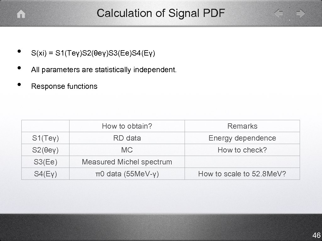Calculation of Signal PDF • • • S(xi) = S 1(Teγ)S 2(θeγ)S 3(Ee)S 4(Eγ) All parameters are statistically independent. Response functions How to obtain? Remarks S 1(Teγ) RD data Energy dependence S 2(θeγ) MC How to check? S 3(Ee) Measured Michel spectrum S 4(Eγ) π0 data (55 Me. V-γ) How to scale to 52. 8 Me. V? 46

Calculation of Signal PDF FWHM 428 ps S 1(Teγ) S 3(Ee) FWHM 0. 96% S 2(θeγ) S 4(Eγ) FWHM 4. 9% 47

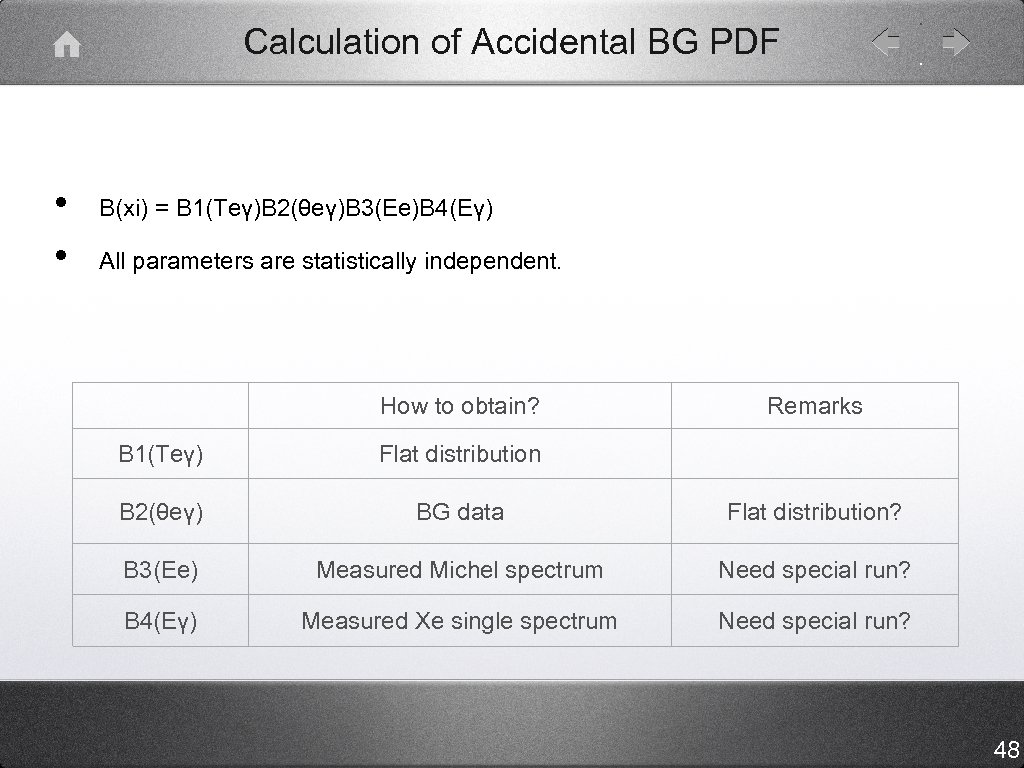Calculation of Accidental BG PDF • • B(xi) = B 1(Teγ)B 2(θeγ)B 3(Ee)B 4(Eγ) All parameters are statistically independent. How to obtain? Remarks B 1(Teγ) Flat distribution B 2(θeγ) BG data Flat distribution? B 3(Ee) Measured Michel spectrum Need special run? B 4(Eγ) Measured Xe single spectrum Need special run? 48

Calculation of Accidental BG PDF B 1(Teγ) B 3(Ee) B 2(θeγ) B 4(Eγ) 49

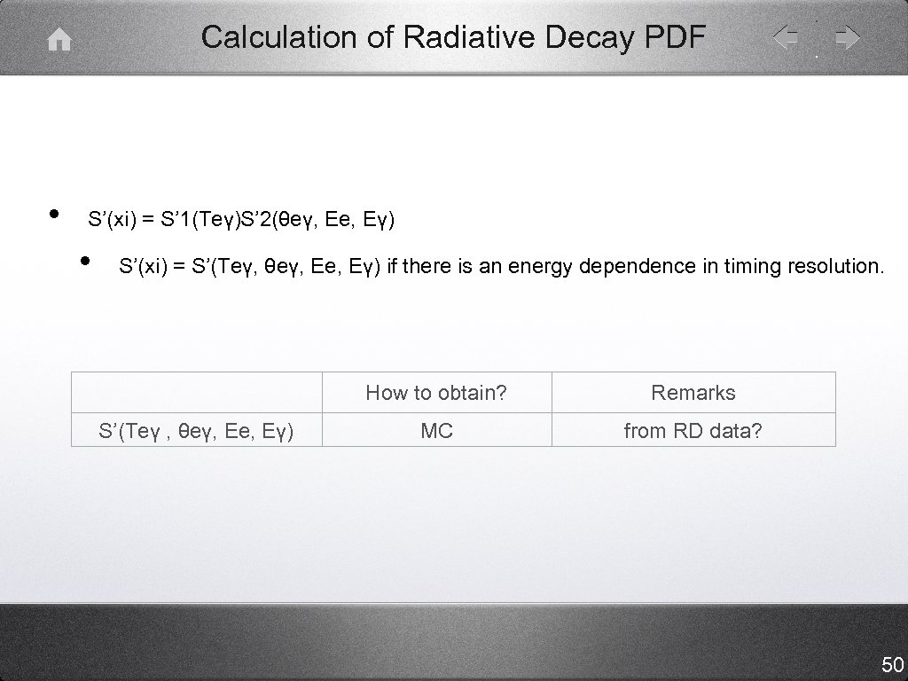Calculation of Radiative Decay PDF • S’(xi) = S’ 1(Teγ)S’ 2(θeγ, Ee, Eγ) • S’(xi) = S’(Teγ, θeγ, Ee, Eγ) if there is an energy dependence in timing resolution. How to obtain? S’(Teγ , θeγ, Ee, Eγ) Remarks MC from RD data? 50

Calculation of Radiative Decay PDF θeγ Ee Ee-Eγ Eγ 51

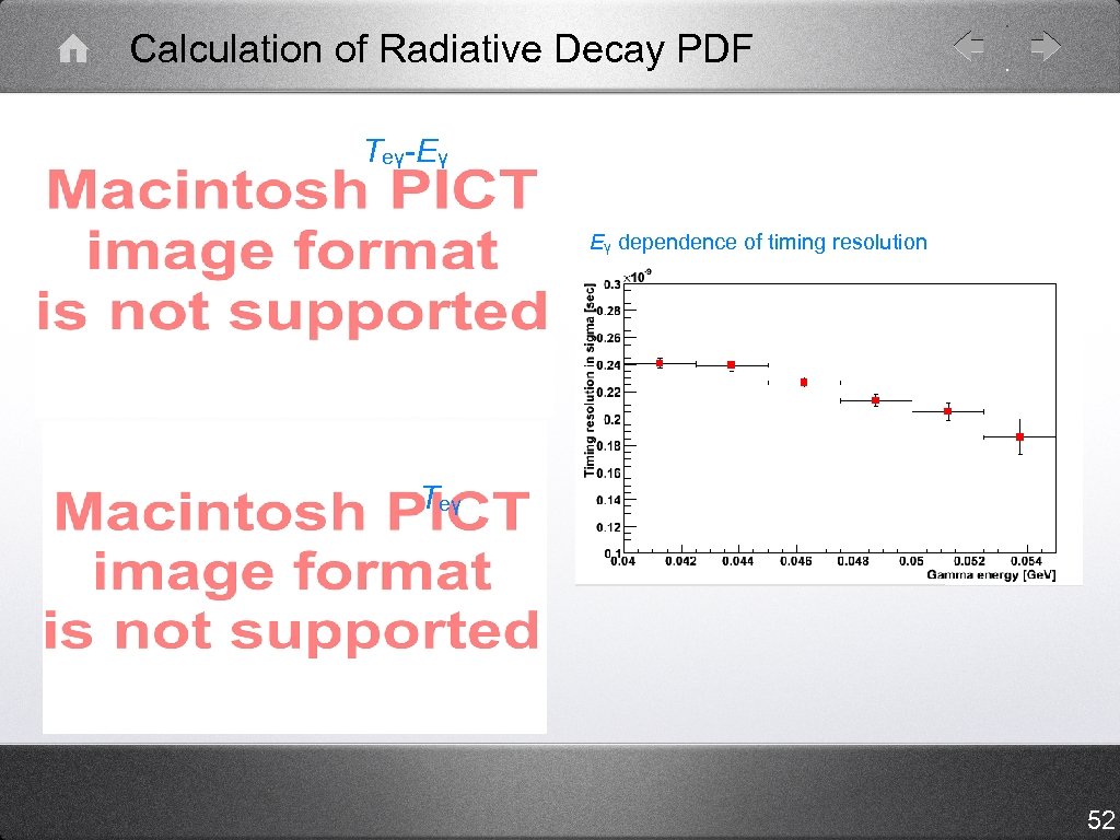Calculation of Radiative Decay PDF Teγ-Eγ Eγ dependence of timing resolution Teγ 52

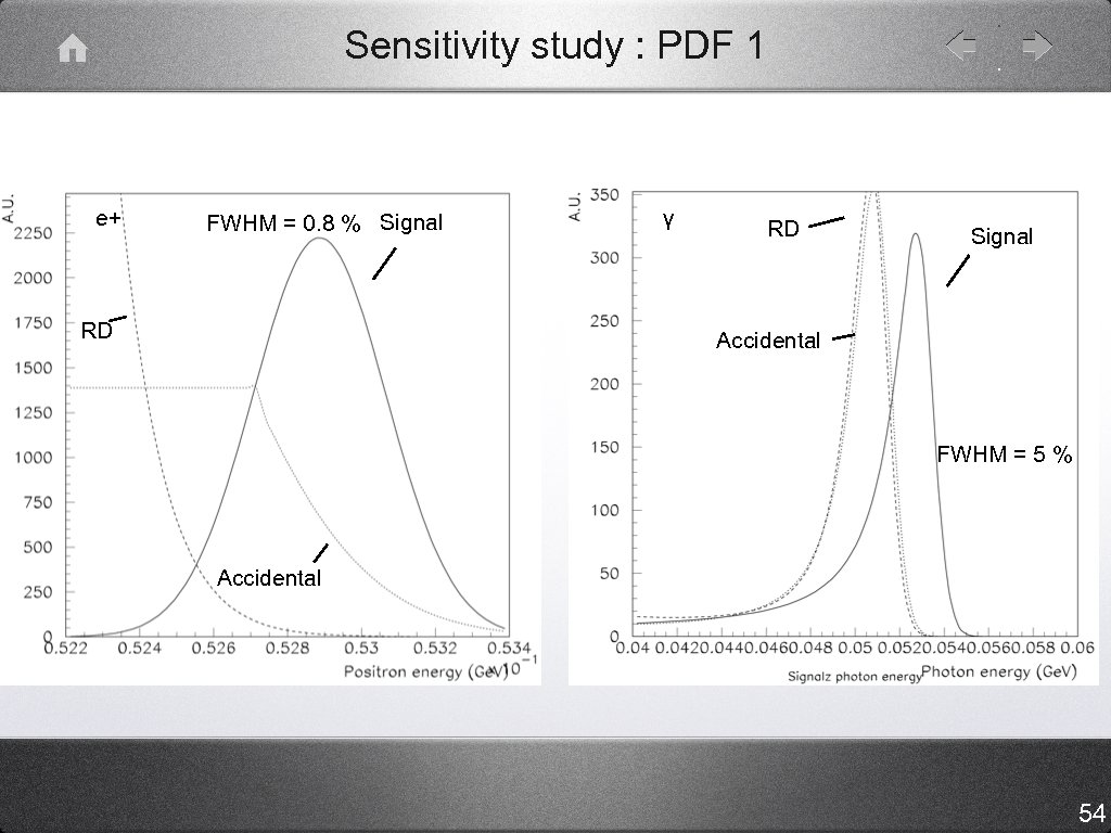
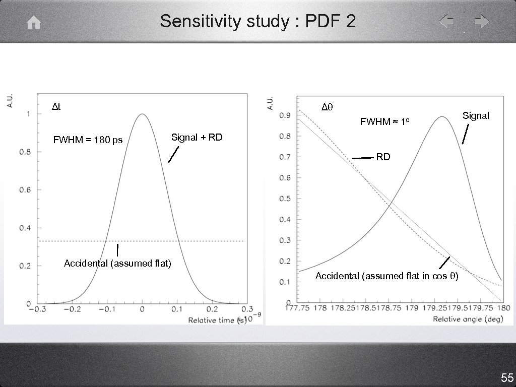
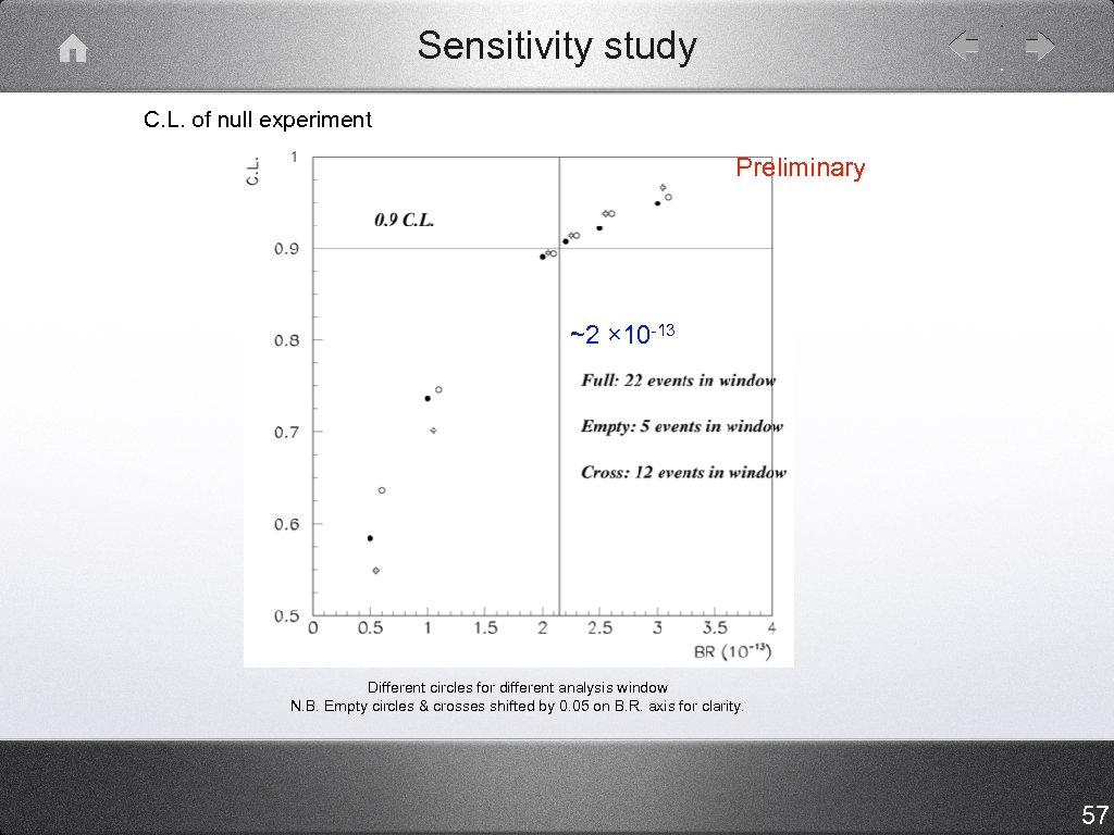
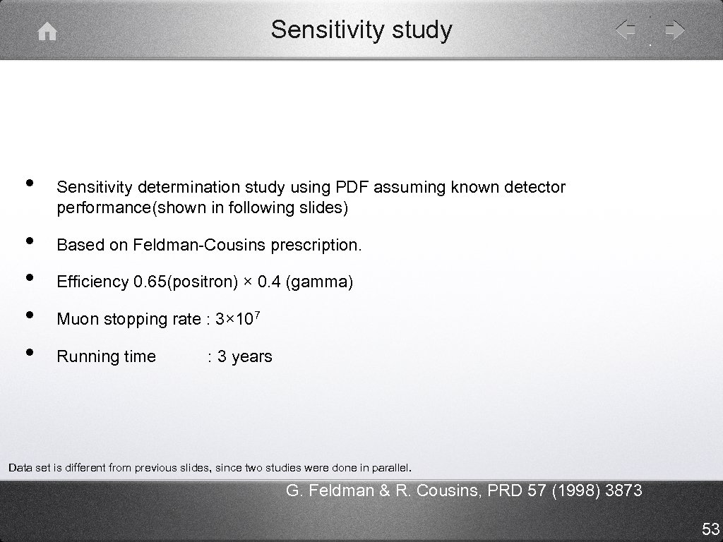Sensitivity study • • • Sensitivity determination study using PDF assuming known detector performance(shown in following slides) Based on Feldman-Cousins prescription. Efficiency 0. 65(positron) × 0. 4 (gamma) Muon stopping rate : 3× 107 Running time : 3 years Data set is different from previous slides, since two studies were done in parallel. G. Feldman & R. Cousins, PRD 57 (1998) 3873 53

Sensitivity study : PDF 1 e+ FWHM = 0. 8 % Signal RD γ RD Signal Accidental FWHM = 5 % Accidental 54

Sensitivity study : PDF 2 Δt Δθ FWHM ≈ 1 o FWHM = 180 ps Signal + RD RD Accidental (assumed flat) Accidental (assumed flat in cos θ) 55

Positron efficiency Scatter TICZ DCH TICP Efficiency % • Event generation (interest region) • • • |ϕ|<60 deg, 0. 08<|cosθ|<0. 35 TC hit definition “Bar” && “Fiber” && “only primary e+” && “ΔXTC < ± 5 cm(Z), ± 3 cm(ϕ) Removed each components one by one “# of accepted e+@TC” / “# of generated e+” Full detector 64. 6 w/o DC system 88. 7 w/o cable duct 66. 1 w/o cable 70. 2 w/o amp 68. 6 w/o frame 77. 6 w/o gas, foil 65. 1 56

Sensitivity study C. L. of null experiment Preliminary ~2 × 10 -13 Different circles for different analysis window N. B. Empty circles & crosses shifted by 0. 05 on B. R. axis for clarity. 57

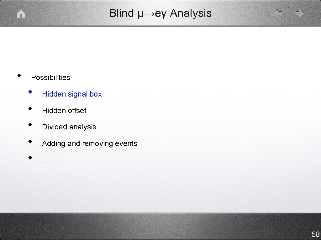Blind μ→eγ Analysis • Possibilities • • • Hidden signal box Hidden offset Divided analysis Adding and removing events. . . 58

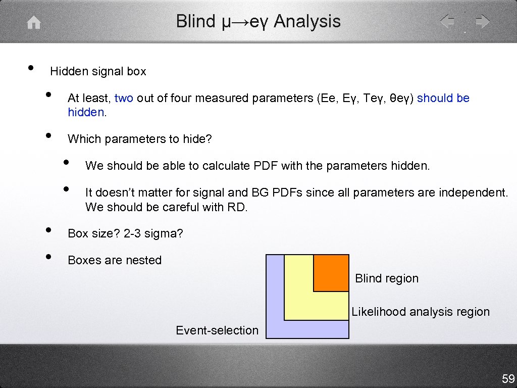Blind μ→eγ Analysis • Hidden signal box • • At least, two out of four measured parameters (Ee, Eγ, Teγ, θeγ) should be hidden. Which parameters to hide? • • We should be able to calculate PDF with the parameters hidden. It doesn’t matter for signal and BG PDFs since all parameters are independent. We should be careful with RD. Box size? 2 -3 sigma? Boxes are nested Blind region Likelihood analysis region Event-selection 59

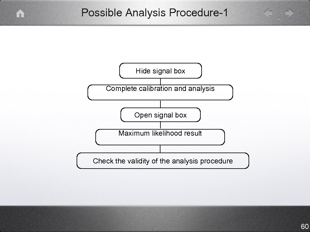Possible Analysis Procedure-1 Hide signal box Complete calibration and analysis Open signal box Maximum likelihood result Check the validity of the analysis procedure 60

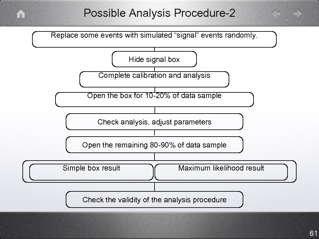Possible Analysis Procedure-2 Replace some events with simulated “signal” events randomly. Hide signal box Complete calibration and analysis Open the box for 10 -20% of data sample Check analysis, adjust parameters Open the remaining 80 -90% of data sample Simple box result Maximum likelihood result Check the validity of the analysis procedure 61

How to Check Analysis Procedure? • • • Compare estimated Nμ→eγ for simulated signal events randomly added in data sample. Compare each single spectrum with likelihood fit result. Compare result on radiative decay with known branching ratio. Re-analyze in subdivided acceptance or subdivided data set. Check the distribution of PDF value. . 62

Computing upgrade • 20 CPUs ➝ 64 CPUs • Need 3 months to become ready after the order • • 2 months for delivery 1 month for setup Upgrade this year in order to buy same nodes as existing ones 26 TBytes ➝ 100 TBytes • • 20 TB for mass production + 6 TB for use = 26 TB Upgrade next year ? • • 20 TB might be enough for this year The later the cheaper 63

Man power • Online S. Ritt, R. Sawada, M. Scheneebeli, G. Signorelli • MC(gem) P. W. Cattaneo, F. Cei, H. Natori, H. Nishiguchi, Y. Nishimura, W. Ootani, V. Tumakov, S. Yamada • MC(bartender) P. W. Cattaneo, Y. Hisamatsu, R. Sawada, V. Tumakov, Y. Uchiyama, S. Yamada • Analysis DCH B. Golden, Y. Hisamatsu, F. Ignatov, W. Molzon, D. Nicolo, H. Nishiguchi, M. Schneebeli, C. Topchan, V. Tumakov, F. Yu, F. Xiao • TC A. Barchiesi, P. W. Cattaneo, G. Cavoto, S. Dussoni, L. Galli, G. Gallucci, Y. Uchiyama, C. Voena • XEC F. Cei, L. Perrozzi, R. Sawada, G. Signorelli, Y. Uchiyama • Physics F. Cei, W. Ootani • People who started contribution to software in this one year, or people who is starting contribution. 64

Summary • Sub-groups in every stages are actively working • • • DAQ, Simulation, Reconstruction and physics People working for software is getting more. Software quality control is getting important Data reduction group is implementing analysis in DAQ. Algorithm depends on subdetectors. Implementation of 3 rd level trigger is also considered Modifications of simulation for performance, and better comparison with analysis result Reconstruction framework of each sub-detectors are getting ready. We are intensively working for improving performance (better resolution, efficiency) Study on procedure of physics analysis is ongoing 65

End