SOES 3015 Lecture Palaeoclimate Models II Model Design

SOES 3015 Lecture Palaeoclimate Models II: Model Design, Data Interpretation & New Hypotheses Bob Marsh

Lecture Overview Ø Throughout the lecture: • How are models used to help interpret palaeodata? • What new hypotheses are supported by models? • What “ideal” models are needed? Ø We’ll look at some modeling case studies: • Abrupt Changes & Cycles in the Quaternary • Pliocene Climate Change as Panama closes • Cenozoic: Antarctic Glaciation • Paleocene-Eocene Thermal Maximum • Snowball Earth: entry & exit

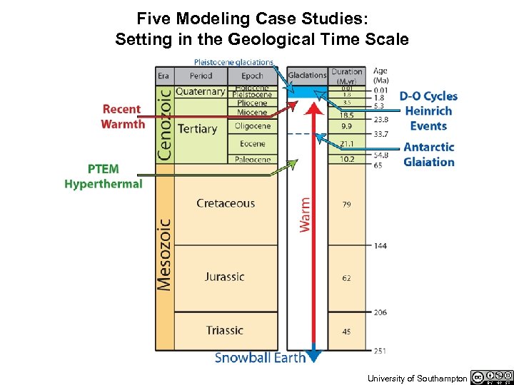Five Modeling Case Studies: Setting in the Geological Time Scale University of Southampton

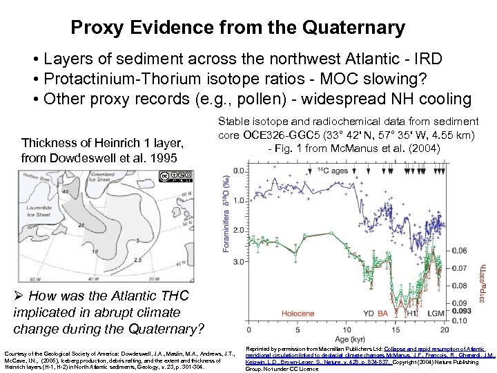Proxy Evidence from the Quaternary • Layers of sediment across the northwest Atlantic - IRD • Protactinium-Thorium isotope ratios - MOC slowing? • Other proxy records (e. g. , pollen) - widespread NH cooling Thickness of Heinrich 1 layer, from Dowdeswell et al. 1995 Stable isotope and radiochemical data from sediment core OCE 326 -GGC 5 (33° 42' N, 57° 35' W, 4. 55 km) - Fig. 1 from Mc. Manus et al. (2004) Ø How was the Atlantic THC implicated in abrupt climate change during the Quaternary? Courtesy of the Geological Society of America: Dowdeswell, J. A. , Maslin, M. A. , Andrews, J. T. , Mc. Cave, I. N. , (2005), Iceberg production, debris rafting, and the extent and thickness of Heinrich layers (H-1, H-2) in North Atlantic sediments, Geology, v. 23, p. 301 -304. Reprinted by permission from Macmillan Publichers Ltd: Collapse and rapid resumption of Atlantic meridional circulation linked to deglacial climate changes Mc. Manus, J. F. , Francois, R. , Gherardi, J. M. , Keigwin, L. D. , Brown-Leger, S. , Nature, v. 428, p. 834 -837, Copyright (2004) Nature Publishing Group. Not under CC Licence

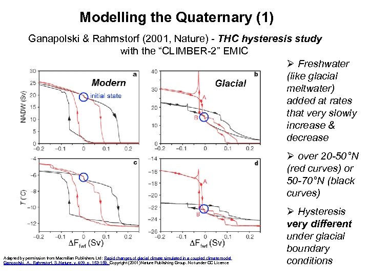Modelling the Quaternary (1) Ganapolski & Rahmstorf (2001, Nature) - THC hysteresis study with the “CLIMBER-2” EMIC Ø Freshwater (like glacial meltwater) added at rates that very slowly increase & decrease Ø over 20 -50°N (red curves) or 50 -70°N (black curves) Adapted by permission from Macmillan Publishers Ltd: Rapid changes of glacial climate simulated in a coupled climate model Ganopolski, A. , Rahmstorf, S. , Nature, v. 409, p. 153 -158. Copyright (2001) Nature Publishing Group. Not under CC Licence Ø Hysteresis very different under glacial boundary conditions

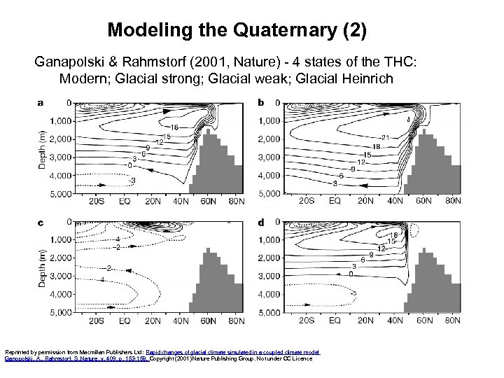Modeling the Quaternary (2) Ganapolski & Rahmstorf (2001, Nature) - 4 states of the THC: Modern; Glacial strong; Glacial weak; Glacial Heinrich Reprinted by permission from Macmillan Publishers Ltd: Rapid changes of glacial climate simulated in a coupled climate model Ganopolski, A. , Rahmstorf, S. , Nature, v. 409, p. 153 -158. Copyright (2001) Nature Publishing Group. Not under CC Licence

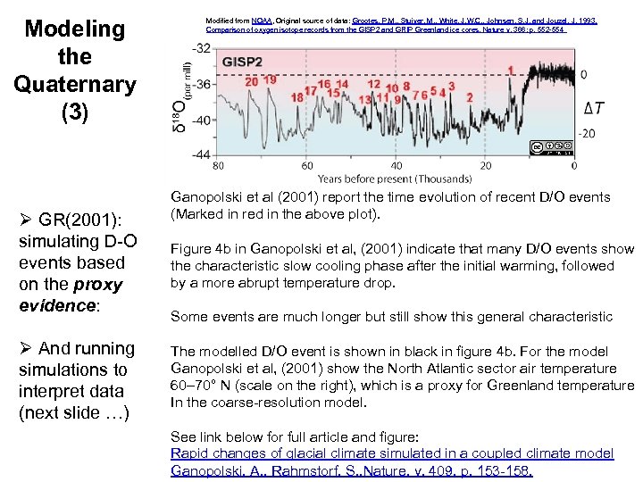Modeling the Quaternary (3) Ø GR(2001): simulating D-O events based on the proxy evidence: Ø And running simulations to interpret data (next slide …) Modified from NOAA, Original source of data: Grootes, P. M. , Stuiver, M. , White, J. W. C. , Johnsen, S. J. and Jouzel, J. 1993. Comparison of oxygen isotope records from the GISP 2 and GRIP Greenland ice cores. Nature v. 366: p. 552 -554 Ganopolski et al (2001) report the time evolution of recent D/O events (Marked in red in the above plot). Figure 4 b in Ganopolski et al, (2001) indicate that many D/O events show the characteristic slow cooling phase after the initial warming, followed by a more abrupt temperature drop. Some events are much longer but still show this general characteristic The modelled D/O event is shown in black in figure 4 b. For the model Ganopolski et al, (2001) show the North Atlantic sector air temperature 60– 70° N (scale on the right), which is a proxy for Greenland temperature In the coarse-resolution model. See link below for full article and figure: Rapid changes of glacial climate simulated in a coupled climate model Ganopolski, A. , Rahmstorf, S. , Nature, v. 409, p. 153 -158.

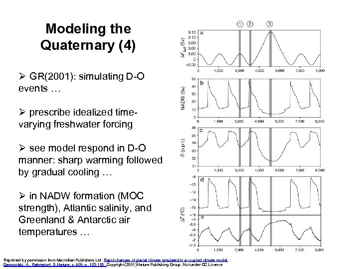Modeling the Quaternary (4) Ø GR(2001): simulating D-O events … Ø prescribe idealized timevarying freshwater forcing Ø see model respond in D-O manner: sharp warming followed by gradual cooling … Ø in NADW formation (MOC strength), Atlantic salinity, and Greenland & Antarctic air temperatures … Reprinted by permission from Macmillan Publishers Ltd: Rapid changes of glacial climate simulated in a coupled climate model Ganopolski, A. , Rahmstorf, S. , Nature, v. 409, p. 153 -158. Copyright (2001) Nature Publishing Group. Not under CC Licence

Modeling the Quaternary (5) Ø GR(2001) and subsequent papers by same authors hypothesize that the stability of the glacial THC was quite different from that of the THC today Ø The modern THC is characterized by more extensive hysteresis: two clear modes (THC on or off) across a wide range of freshwater forcing Ø But the glacial THC is close to a “warm mode”: if net evaporation increases slightly in the subtropics / mid-lats, THC intensity may increase by O(10 Sv) Ø Further experiments implicate the varying THC (and associated heat transport) in D-O cycles

Modeling the Quaternary (6) Ø Focus on the last deglaciation (next six slides) Ø “In Progress” GENIE study (Marsh, Rohling, et al. ) Ø To model the Atlantic Overturning since 21 ka BP Ø Paying special attention to the details of ice sheet melting & the low-latitude hydrological cycle Ø Ultimately to capture three events: Heinrich Event 1 (~16 ka); the Bølling Allerød (~14. 5 ka); the Younger Dryas (~12. 5 ka)

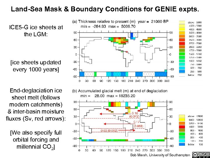Land-Sea Mask & Boundary Conditions for GENIE expts. ICE 5 -G ice sheets at the LGM: [ice sheets updated every 1000 years] End-deglaciation ice sheet melt (follows modern catchments) & inter-basin moisture fluxes (Sv, red arrows): [We also specify full orbital forcing and millennial CO 2] Bob Marsh, University of Southampton

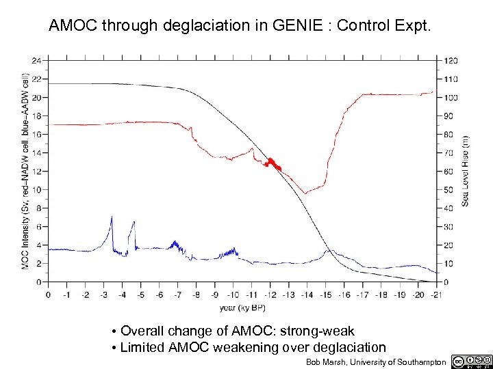AMOC through deglaciation in GENIE : Control Expt. • Overall change of AMOC: strong-weak • Limited AMOC weakening over deglaciation Bob Marsh, University of Southampton

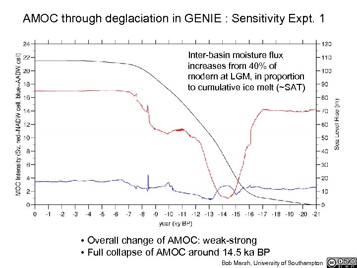AMOC through deglaciation in GENIE : Sensitivity Expt. 1 Inter-basin moisture flux increases from 40% of modern at LGM, in proportion to cumulative ice melt (~SAT) • Overall change of AMOC: weak-strong • Full collapse of AMOC around 14. 5 ka BP Bob Marsh, University of Southampton

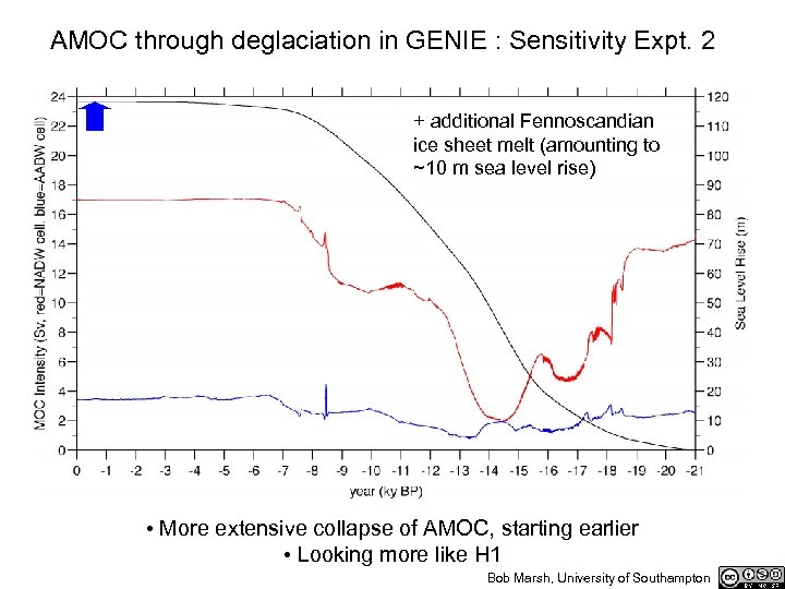AMOC through deglaciation in GENIE : Sensitivity Expt. 2 + additional Fennoscandian ice sheet melt (amounting to ~10 m sea level rise) • More extensive collapse of AMOC, starting earlier • Looking more like H 1 Bob Marsh, University of Southampton

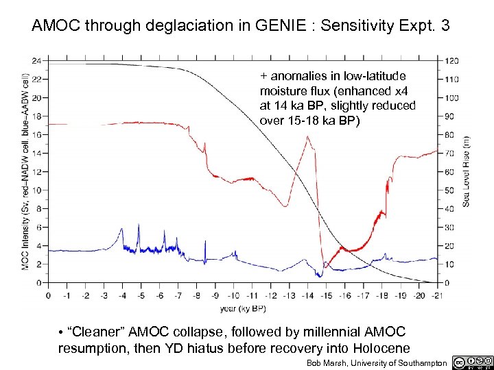AMOC through deglaciation in GENIE : Sensitivity Expt. 3 + anomalies in low-latitude moisture flux (enhanced x 4 at 14 ka BP, slightly reduced over 15 -18 ka BP) • “Cleaner” AMOC collapse, followed by millennial AMOC resumption, then YD hiatus before recovery into Holocene Bob Marsh, University of Southampton

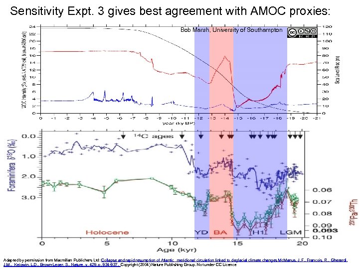Sensitivity Expt. 3 gives best agreement with AMOC proxies: Bob Marsh, University of Southampton Adapted by permission from Macmillan Publichers Ltd: Collapse and rapid resumption of Atlantic meridional circulation linked to deglacial climate changes Mc. Manus, J. F. , Francois, R. , Gherardi, J. M. , Keigwin, L. D. , Brown-Leger, S. , Nature, v. 428, p. 834 -837, Copyright (2004) Nature Publishing Group. Not under CC Licence

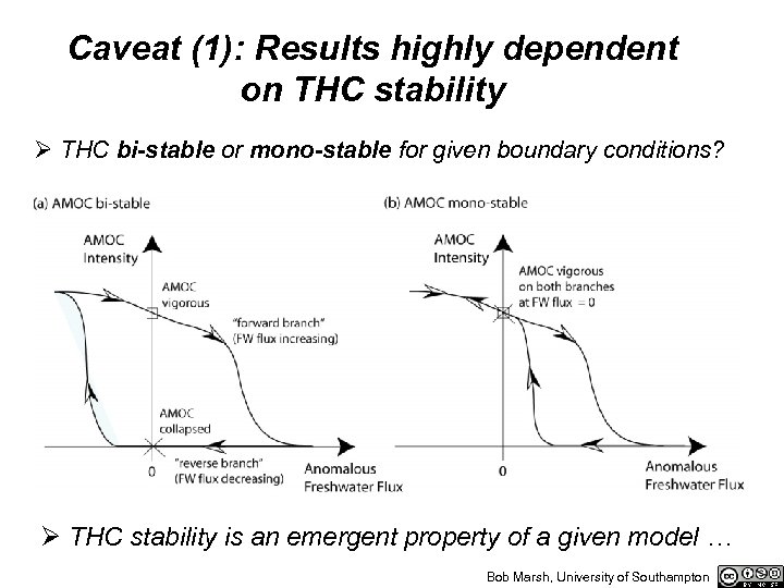Caveat (1): Results highly dependent on THC stability Ø THC bi-stable or mono-stable for given boundary conditions? Ø THC stability is an emergent property of a given model … Bob Marsh, University of Southampton

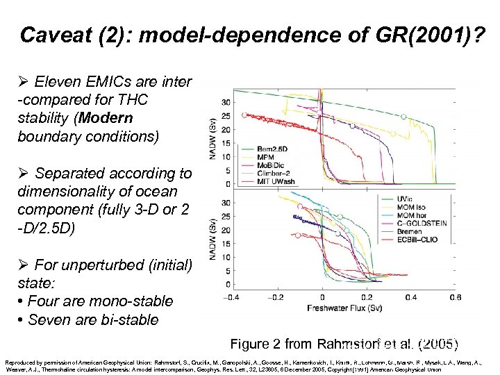Caveat (2): model-dependence of GR(2001)? Ø Eleven EMICs are inter -compared for THC stability (Modern boundary conditions) Ø Separated according to dimensionality of ocean component (fully 3 -D or 2 -D/2. 5 D) Ø For unperturbed (initial) state: • Four are mono-stable • Seven are bi-stable Figure 2 from Rahmstorf et al. (2005) Reproduced by permission of American Geophysical Union: Miller, K. G. , Wright, J. D. , Fairbanks, G. G. , Unlocking the Ice House: Oligocene-Miocene Oxygen Isotopes, Eustasy, and Margin Erosion, J. Geophys. Res. , v. 96(B 4), p. 6829– 6848. Reproduced by permission of American Geophysical Union: Rahmstorf, S. , Crucifix, M. , Ganopolski, A. , Goosse, H. , Kamenkovich, I. , Knutti, R. , Lohmann, G. , Marsh, R. , Mysak, L. A. , Wang, A. , 6 August 1990. Copyright [1991] American Geophysical Union Weaver, A. J. , Thermohaline circulation hysteresis: A model intercomparison, Geophys. Res. Lett. , 32, L 23605, 6 December 2005, Copyright [1991] American Geophysical Union

Beyond GR(2001): How to model Heinrich Events & their paleo-record? Ø Components in addition to basic climate model: ice sheet, icebergs, including sediment transport and deposition module Ø With boundary conditions: glacial CO 2; orbital parameters; initial ice sheets (e. g. , LGM, allowed to subsequently vary) Ø To capture: “binge-purge” oscillation of Laurentide and/or Fennoscandian ice sheet; massive iceberg calving; progressive iceberg melting & corresponding deposition of terrestrial sediment; freshwater influence on thermohaline circulation Ø On timescales from annual to millennial; coupled feedbacks involving the atmosphere and sea ice, on timescales from seasonal to decadal

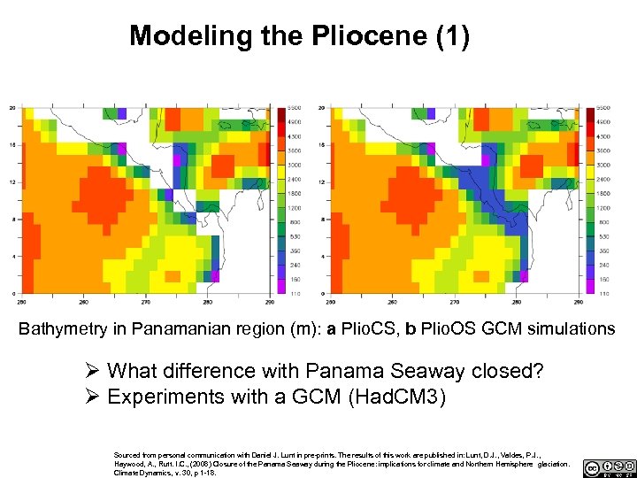Modeling the Pliocene (1) Bathymetry in Panamanian region (m): a Plio. CS, b Plio. OS GCM simulations Ø What difference with Panama Seaway closed? Ø Experiments with a GCM (Had. CM 3) Sourced from personal communication with Daniel J. Lunt in pre-prints. The results of this work are published in: Lunt, D. J. , Valdes, P. J. , Haywood, A. , Rutt. I. C. , (2008) Closure of the Panama Seaway during the Pliocene: implications for climate and Northern Hemisphere glaciation. Climate Dynamics, v. 30, p 1 -18.

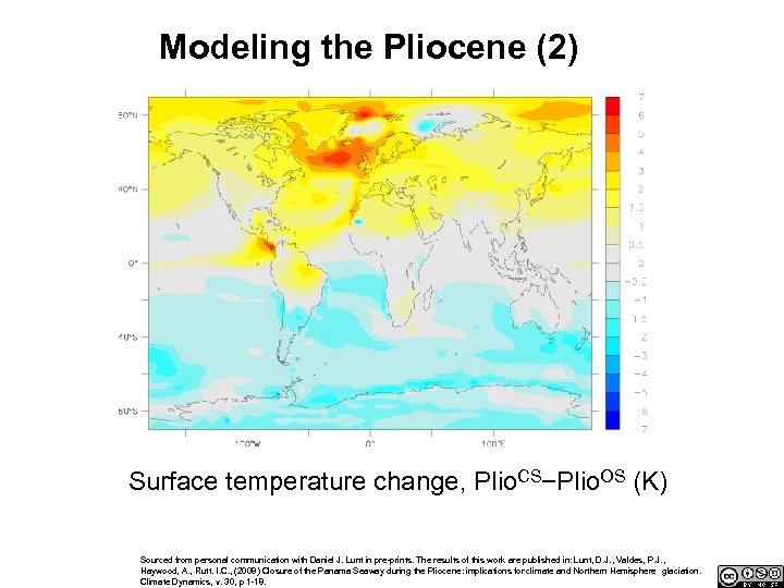Modeling the Pliocene (2) Surface temperature change, Plio. CS−Plio. OS (K) Sourced from personal communication with Daniel J. Lunt in pre-prints. The results of this work are published in: Lunt, D. J. , Valdes, P. J. , Haywood, A. , Rutt. I. C. , (2008) Closure of the Panama Seaway during the Pliocene: implications for climate and Northern Hemisphere glaciation. Climate Dynamics, v. 30, p 1 -18.

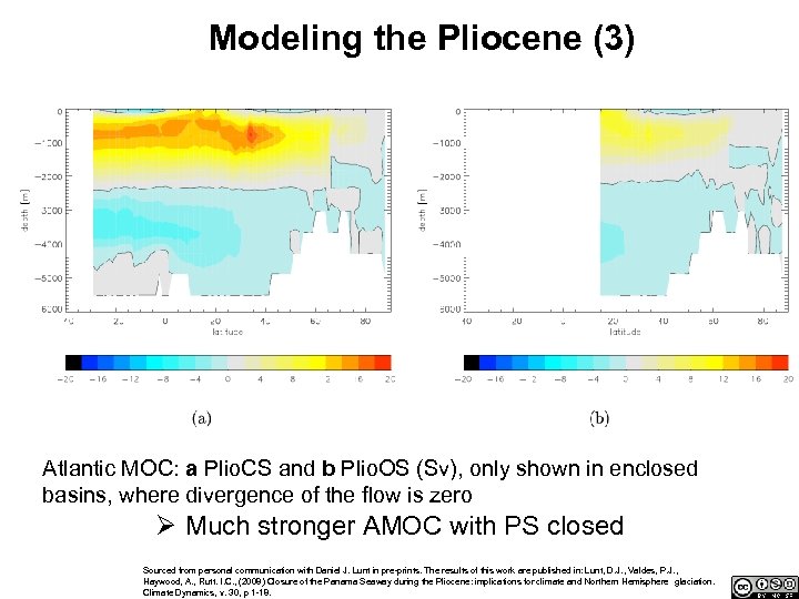Modeling the Pliocene (3) Atlantic MOC: a Plio. CS and b Plio. OS (Sv), only shown in enclosed basins, where divergence of the flow is zero Ø Much stronger AMOC with PS closed Sourced from personal communication with Daniel J. Lunt in pre-prints. The results of this work are published in: Lunt, D. J. , Valdes, P. J. , Haywood, A. , Rutt. I. C. , (2008) Closure of the Panama Seaway during the Pliocene: implications for climate and Northern Hemisphere glaciation. Climate Dynamics, v. 30, p 1 -18.

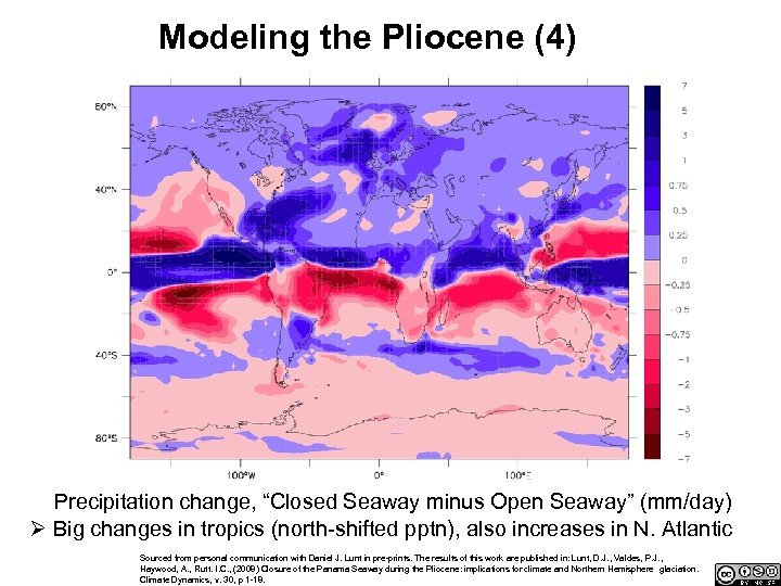Modeling the Pliocene (4) Precipitation change, “Closed Seaway minus Open Seaway” (mm/day) Ø Big changes in tropics (north-shifted pptn), also increases in N. Atlantic Sourced from personal communication with Daniel J. Lunt in pre-prints. The results of this work are published in: Lunt, D. J. , Valdes, P. J. , Haywood, A. , Rutt. I. C. , (2008) Closure of the Panama Seaway during the Pliocene: implications for climate and Northern Hemisphere glaciation. Climate Dynamics, v. 30, p 1 -18.

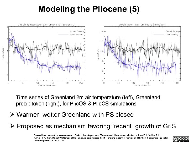Modeling the Pliocene (5) Time series of Greenland 2 m air temperature (left), Greenland precipitation (right), for Plio. OS & Plio. CS simulations Ø Warmer, wetter Greenland with PS closed Ø Proposed as mechanism favoring “recent” growth of Gr. IS Sourced from personal communication with Daniel J. Lunt in pre-prints. The results of this work are published in: Lunt, D. J. , Valdes, P. J. , Haywood, A. , Rutt. I. C. , (2008) Closure of the Panama Seaway during the Pliocene: implications for climate and Northern Hemisphere glaciation. Climate Dynamics, v. 30, p 1 -18.

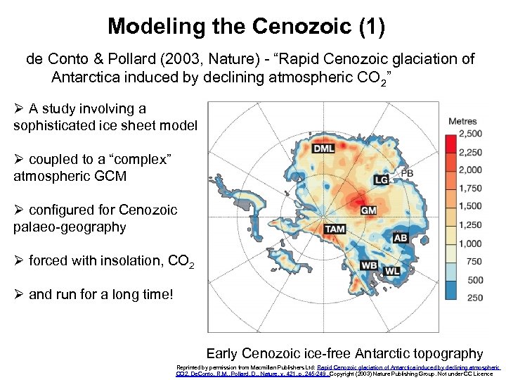Modeling the Cenozoic (1) de Conto & Pollard (2003, Nature) - “Rapid Cenozoic glaciation of Antarctica induced by declining atmospheric CO 2” Ø A study involving a sophisticated ice sheet model Ø coupled to a “complex” atmospheric GCM Ø configured for Cenozoic palaeo-geography Ø forced with insolation, CO 2 Ø and run for a long time! Early Cenozoic ice-free Antarctic topography Reprinted by permission from Macmillan Publishers Ltd: Rapid Cenozoic glaciation of Antarctica induced by declining atmospheric CO 2, De. Conto, R. M. , Pollard, D. , Nature, v. 421, p. 245 -249. Copyright (2003) Nature Publishing Group. Not under CC Licence

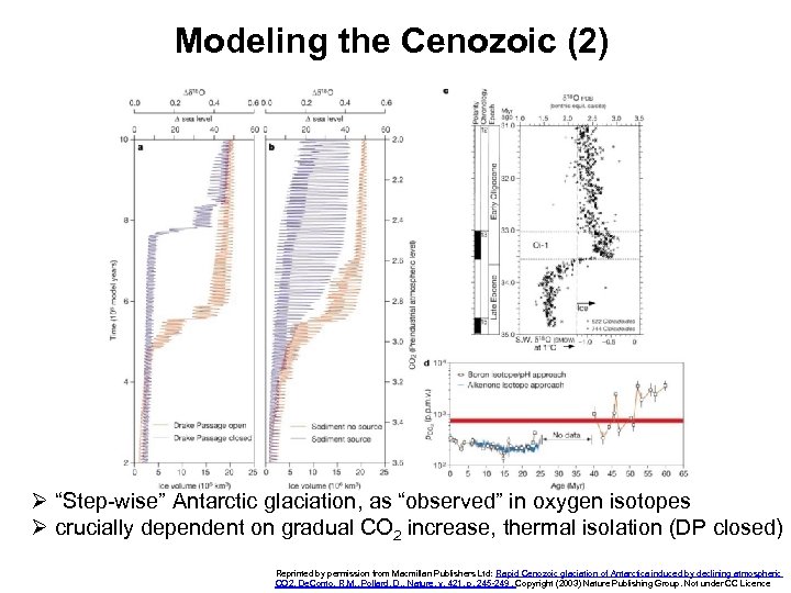Modeling the Cenozoic (2) Ø “Step-wise” Antarctic glaciation, as “observed” in oxygen isotopes Ø crucially dependent on gradual CO 2 increase, thermal isolation (DP closed) Reprinted by permission from Macmillan Publishers Ltd: Rapid Cenozoic glaciation of Antarctica induced by declining atmospheric CO 2, De. Conto, R. M. , Pollard, D. , Nature, v. 421, p. 245 -249. Copyright (2003) Nature Publishing Group. Not under CC Licence

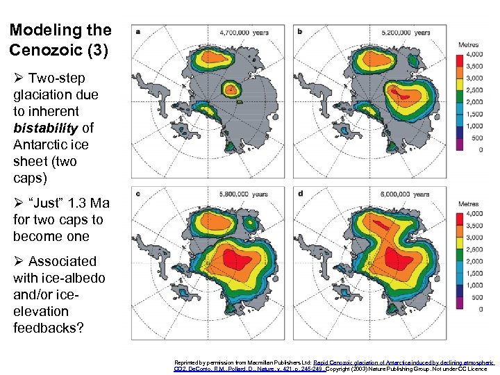Modeling the Cenozoic (3) Ø Two-step glaciation due to inherent bistability of Antarctic ice sheet (two caps) Ø “Just” 1. 3 Ma for two caps to become one Ø Associated with ice-albedo and/or iceelevation feedbacks? Reprinted by permission from Macmillan Publishers Ltd: Rapid Cenozoic glaciation of Antarctica induced by declining atmospheric CO 2, De. Conto, R. M. , Pollard, D. , Nature, v. 421, p. 245 -249. Copyright (2003) Nature Publishing Group. Not under CC Licence

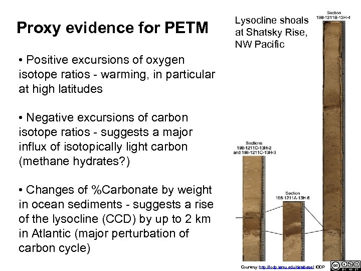Proxy evidence for PETM Lysocline shoals at Shatsky Rise, NW Pacific • Positive excursions of oxygen isotope ratios - warming, in particular at high latitudes • Negative excursions of carbon isotope ratios - suggests a major influx of isotopically light carbon (methane hydrates? ) • Changes of %Carbonate by weight in ocean sediments - suggests a rise of the lysocline (CCD) by up to 2 km in Atlantic (major perturbation of carbon cycle) Courtesy: http: //iodp. tamu. edu/database/ IODP

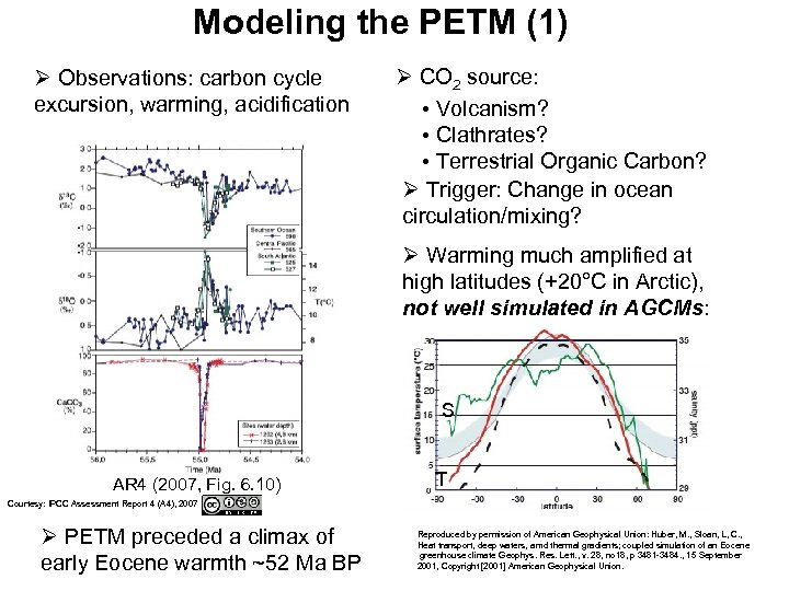Modeling the PETM (1) Ø Observations: carbon cycle excursion, warming, acidification Ø CO 2 source: • Volcanism? • Clathrates? • Terrestrial Organic Carbon? Ø Trigger: Change in ocean circulation/mixing? Ø Warming much amplified at high latitudes (+20°C in Arctic), not well simulated in AGCMs: S AR 4 (2007, Fig. 6. 10) T Courtesy: IPCC Assessment Report 4 (A 4), 2007 Ø PETM preceded a climax of early Eocene warmth ~52 Ma BP Reproduced by permission of American Geophysical Union: Huber, M. , Sloan, L, C. , Heat transport, deep waters, amd thermal gradients; coupled simulation of an Eocene greenhouse climate Geophys. Res. Lett. , v. 28, no 18, p 3481 -3484. , 15 September 2001, Copyright [2001] American Geophysical Union.

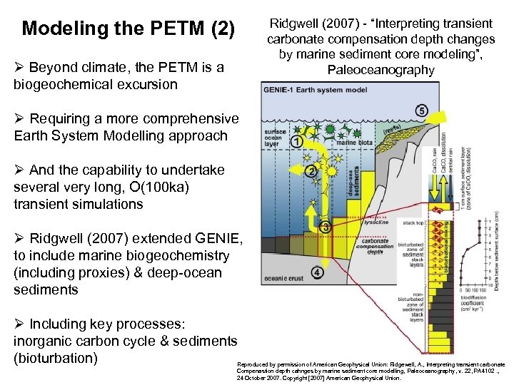Ridgwell (2007) - “Interpreting transient carbonate compensation depth changes by marine sediment core modeling”, Paleoceanography Modeling the PETM (2) Ø Beyond climate, the PETM is a biogeochemical excursion Ø Requiring a more comprehensive Earth System Modelling approach Ø And the capability to undertake several very long, O(100 ka) transient simulations Ø Ridgwell (2007) extended GENIE, to include marine biogeochemistry (including proxies) & deep-ocean sediments Ø Including key processes: inorganic carbon cycle & sediments (bioturbation) Reproduced by permission of American Geophysical Union: Ridgewell, A. , Interpreting transient carbonate Compenastion depth cahnges by marine sediment core modelling, Paleoceanography, v. 22, PA 4102. , 24 October 2007. Copyright [2007] American Geophysical Union.

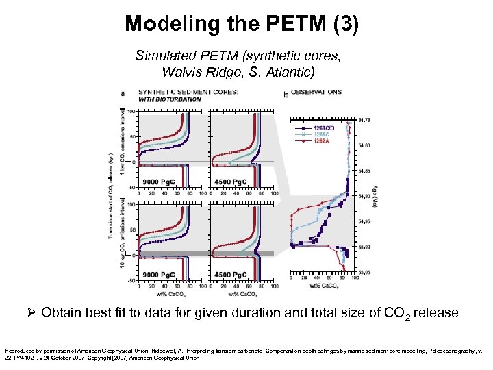Modeling the PETM (3) Simulated PETM (synthetic cores, Walvis Ridge, S. Atlantic) Ø Obtain best fit to data for given duration and total size of CO 2 release Reproduced by permission of American Geophysical Union: Ridgewell, A. , Interpreting transient carbonate Compenastion depth cahnges by marine sediment core modelling, Paleoceanography, v. 22, PA 4102. , v 24 October 2007. Copyright [2007] American Geophysical Union.

Ingredients for comprehensive EMIC modeling of the PETM? Ø Components additional to basic climate model: marine & terrestrial biogeochemistry; ocean sediments (incl. diagenesis); methane hydrate distribution (from “stand-alone” model) Ø Plus boundary conditions: paleo-geography and topography (including catchment areas); initially 3 x present day CO 2; winds from an AGCM for the late Paleocene (if EMIC) Ø To capture: trigger mechanism (e. g. , methane release) on timescale of millennia; near-instant response of global climate system to perturbed radiative forcing; adjustment of ocean circulation, on decadal-millennial timescales; response of terrestrial & marine carbon cycles (especially calcite compensation depth in ocean), over decades-millennia

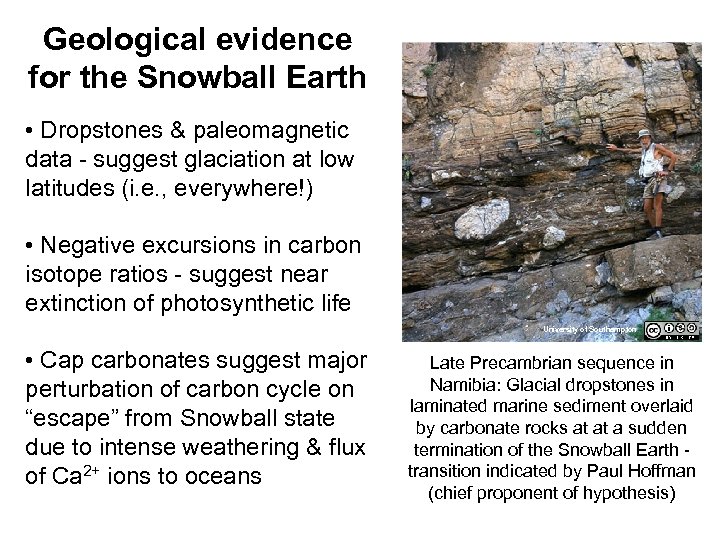Geological evidence for the Snowball Earth • Dropstones & paleomagnetic data - suggest glaciation at low latitudes (i. e. , everywhere!) • Negative excursions in carbon isotope ratios - suggest near extinction of photosynthetic life University of Southampton • Cap carbonates suggest major perturbation of carbon cycle on “escape” from Snowball state due to intense weathering & flux of Ca 2+ ions to oceans Late Precambrian sequence in Namibia: Glacial dropstones in laminated marine sediment overlaid by carbonate rocks at at a sudden termination of the Snowball Earth - transition indicated by Paul Hoffman (chief proponent of hypothesis)

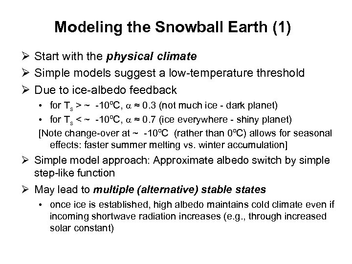Modeling the Snowball Earth (1) Ø Start with the physical climate Ø Simple models suggest a low-temperature threshold Ø Due to ice-albedo feedback • for Ts > ~ -10ºC, ≈ 0. 3 (not much ice - dark planet) • for Ts < ~ -10ºC, ≈ 0. 7 (ice everywhere - shiny planet) [Note change-over at ~ -10ºC (rather than 0ºC) allows for seasonal effects: faster summer melting vs. winter accumulation] Ø Simple model approach: Approximate albedo switch by simple step-like function Ø May lead to multiple (alternative) stable states • once is established, high albedo maintains cold climate even if incoming shortwave radiation increases (e. g. , through increased solar constant)

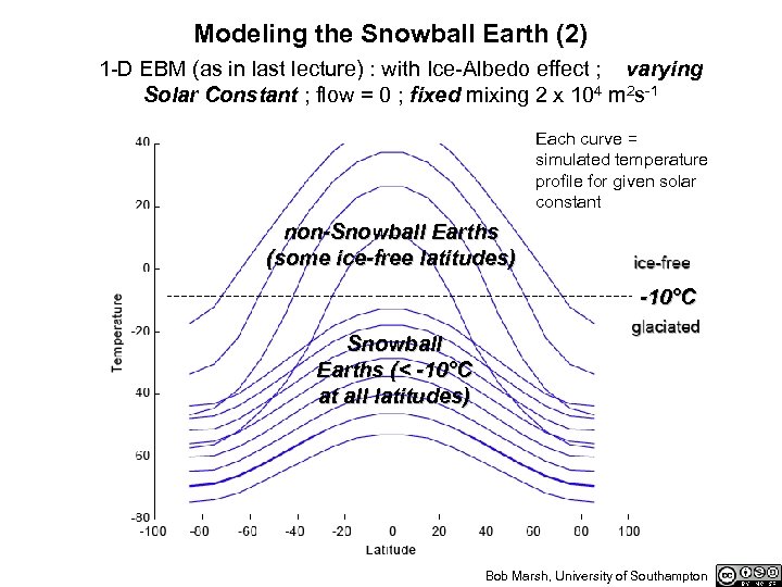Modeling the Snowball Earth (2) 1 -D EBM (as in last lecture) : with Ice-Albedo effect ; varying Solar Constant ; flow = 0 ; fixed mixing 2 x 104 m 2 s-1 Each curve = simulated temperature profile for given solar constant non-Snowball Earths (some ice-free latitudes) -10°C Snowball Earths (< -10°C at all latitudes) Bob Marsh, University of Southampton

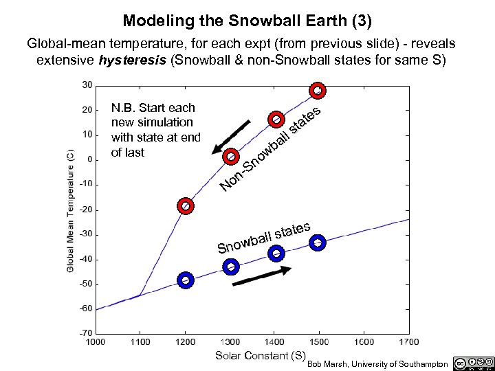Modeling the Snowball Earth (3) Global-mean temperature, for each expt (from previous slide) - reveals extensive hysteresis (Snowball & non-Snowball states for same S) N. B. Start each new simulation with state at end of last s te a st l al wb no S n. No tes ll sta a nowb S Solar Constant (S) Bob Marsh, University of Southampton

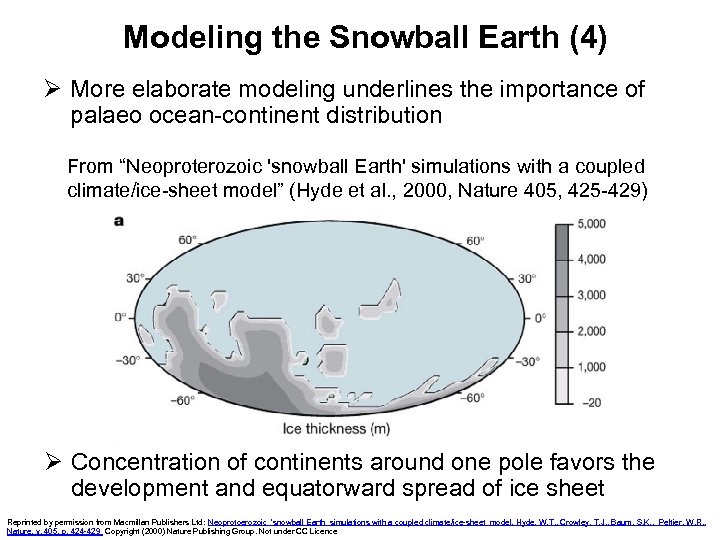Modeling the Snowball Earth (4) Ø More elaborate modeling underlines the importance of palaeo ocean-continent distribution From “Neoproterozoic 'snowball Earth' simulations with a coupled climate/ice-sheet model” (Hyde et al. , 2000, Nature 405, 425 -429) Ø Concentration of continents around one pole favors the development and equatorward spread of ice sheet Reprinted by permission from Macmillan Publishers Ltd: Neoprotoerozoic ‘snowball Earth simulations with a coupled climate/ice-sheet model, Hyde, W. T. , Crowley, T. J. , Baum, S. K. , Peltier, W. R. , Nature, v. 405, p. 424 -429 Copyright (2000) Nature Publishing Group. Not under CC Licence

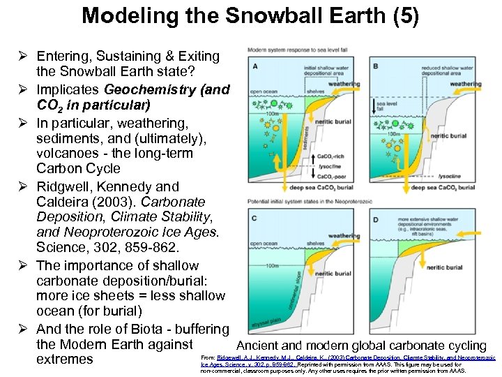Modeling the Snowball Earth (5) Ø Entering, Sustaining & Exiting the Snowball Earth state? Ø Implicates Geochemistry (and CO 2 in particular) Ø In particular, weathering, sediments, and (ultimately), volcanoes - the long-term Carbon Cycle Ø Ridgwell, Kennedy and Caldeira (2003). Carbonate Deposition, Climate Stability, and Neoproterozoic Ice Ages. Science, 302, 859 -862. Ø The importance of shallow carbonate deposition/burial: more ice sheets = less shallow ocean (for burial) Ø And the role of Biota - buffering the Modern Earth against Ancient and modern global carbonate cycling extremes From: Ridgewell, A. J. , Kennedy, M. J. , Caldeira, K. , (2003) Carbonate Deposition, Cliamte Stability, and Neoproterozoic Ice Ages, Science, v. 302, p. 859 -862. Reprinted with permission from AAAS. This figure may be used for non-commercial, classroom purposes only. Any other uses requires the prior written permission from AAAS.

Modeling the Snowball Earth (6) Ø How to model all this? Ø Start simple! Ø Ridgwell et al. (2003) used the PANDORA ocean carbon cycle box model (developed by Wally Broecker), coupled to a representation of the preservation and burial of Ca. CO 3 in deep-sea sediments Ø They provided long-term negative feedback by specifying weathering fluxes of carbon (15 Tmol year– 1) and alkalinity (40 Tmol year– 1), based on estimates for a world before the appearance of vascular plants Ø They left volcanic CO 2 outgassing (5 Tmol year– 1) constant Ø They thus calculated the evolution in atmospheric CO 2 that arises from a reduction in the area available for neritic carbonate deposition (through the Snowball glaciation)

“Ultimate” model of Snowball Earth entry (glaciation) and exit (deglaciation) Ø Components additional to basic climate model: ice sheets; marine & terrestrial (bio? )geochemistry; ocean sediments; lithosphere (weathering); volcanic CO 2 emissions Ø With boundary conditions: varying solar constant, orbital parameters and/or atmospheric CO 2 (to trigger glaciation); neo-Proterozoic distribution of land, perhaps concentrated in low latitudes or one hemisphere Ø Capturing: ice-albedo feedback and associated bistability (Snowball or non-Snowball state); slow carbon cycle (weathering balancing volcanic emissions), on 100 x millennial timescales!

Summary Ø Why model palaeoclimate? • • • For more fundamental understanding of climate system To help interpret proxies To inform us about the Anthropocene - Latest Assessment Report (AR 4) features Paleoclimate chapter, for the first time Ø Different models for different problems • • • Simple Equations (Ridgwell et al. 2003; Hansen et al. 2007 - see last lecture) EMICs (Ganapolski & Rahmstorf 2001; Ridgwell 2007) OAGCMs (Hyde et al. 2000; de. Conto & Pollard 2003; Lunt et al. 2008) Ø Five Case Studies: Quaternary; Pliocene; Cenozoic; PETM; Snowball Earth (each with a different model)

Monday (3 -6 pm, Mon 8 March) Ø The GENIE model has been recently adapted for teaching by colleagues at the Open University Ø The application runs under Windows, and is installed on the machines in 121/02 Ø Please be in 121/02 at 3 pm (as scheduled), where you can work from an instruction sheet (2 -3 instructors on hand to provide advice to individuals) Ø Then work individually or in pairs, running GENIE in a small range of palaeo-flavoured experiments Ø The practical is designed to give you some direct experience of: • • • what an EMIC looks like how fast it runs the kind of data (plots) that are produced

Copyright statement • This resource was created by the University of Southampton and released as an open educational resource through the 'C -change in GEES' project exploring the open licensing of climate change and sustainability resources in the Geography, Earth and Environmental Sciences. The C-change in GEES project was funded by HEFCE as part of the JISC/HE Academy UKOER programme and coordinated by the GEES Subject Centre. • This resource is licensed under the terms of the Attribution-Non-Commercial-Share Alike 2. 0 UK: England & Wales license (http: //creativecommons. org/licenses/by-nc-sa/2. 0/uk/). • However the resource, where specified below, contains other 3 rd party materials under their own licenses. The licenses and attributions are outlined below: • The University of Southampton and the National Oceanography Centre, Southampton and its logos are registered trade marks of the University. The University reserves all rights to these items beyond their inclusion in these CC resources. • The JISC logo, the C-change logo and the logo of the Higher Education Academy Subject Centre for the Geography, Earth and Environmental Sciences are licensed under the terms of the Creative Commons Attribution -non-commercial-No Derivative Works 2. 0 UK England & Wales license. All reproductions must comply with the terms of that license. • All content reproduced from copyrighted material of the American Geophysical Union (AGU) are subject to the terms and conditions as published at: http: //www. agu. org/pubs/authors/usage_permissions. shtml AGU content may be reproduced and modified for non-commercial and classroom use only. Any other use requires the prror written permission from AGU. • All content reproduced from the American Association for the Advancement of Science (AAAS) may be reproduced for non commercial classroom purposes only, any other uses requires the prior written permission from AAAS. • All content reproduced from Macmillan Publishers Ltd remains the copyright of Macmillan Publishers Ltd. Reproduction of copyrighted material is permitted for noncommercial personal and/or classroom use only. Any other use requires the prior written permission of Macmillan Publishers Ltd