Slides for Introduction to Stochastic Search and Optimization

Slides for Introduction to Stochastic Search and Optimization (ISSO) by J. C. Spall CHAPTER 1 STOCHASTIC SEARCH AND OPTIMIZATION: MOTIVATION AND SUPPORTING RESULTS • Organization of chapter in ISSO –Introduction –Some principles of stochastic search and optimization • Key points in implementation and analysis • No free lunch theorems –Gradients, Hessians, etc. –Steepest descent and Newton-Raphson search

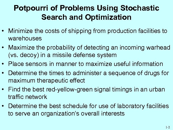Potpourri of Problems Using Stochastic Search and Optimization • Minimize the costs of shipping from production facilities to warehouses • Maximize the probability of detecting an incoming warhead (vs. decoy) in a missile defense system • Place sensors in manner to maximize useful information • Determine the times to administer a sequence of drugs for maximum therapeutic effect • Find the best red-yellow-green signal timings in an urban traffic network • Determine the best schedule for use of laboratory facilities to serve an organization’s overall interests 1 -2

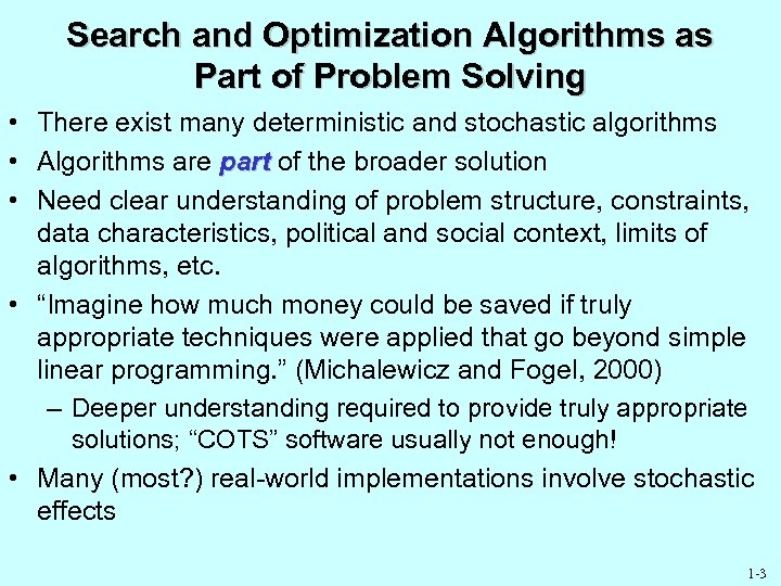Search and Optimization Algorithms as Part of Problem Solving • There exist many deterministic and stochastic algorithms • Algorithms are part of the broader solution • Need clear understanding of problem structure, constraints, data characteristics, political and social context, limits of algorithms, etc. • “Imagine how much money could be saved if truly appropriate techniques were applied that go beyond simple linear programming. ” (Michalewicz and Fogel, 2000) – Deeper understanding required to provide truly appropriate solutions; “COTS” software usually not enough! • Many (most? ) real-world implementations involve stochastic effects 1 -3

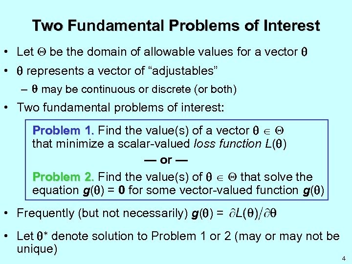Two Fundamental Problems of Interest • Let be the domain of allowable values for a vector • represents a vector of “adjustables” – may be continuous or discrete (or both) • Two fundamental problems of interest: Problem 1. Find the value(s) of a vector that minimize a scalar-valued loss function L( ) — or — Problem 2. Find the value(s) of that solve the equation g( ) = 0 for some vector-valued function g( ) • Frequently (but not necessarily) g( ) = • Let denote solution to Problem 1 or 2 (may or may not be unique) 4

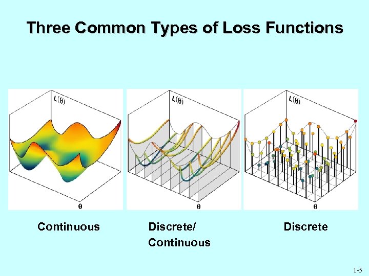Three Common Types of Loss Functions Continuous Discrete/ Continuous Discrete 1 -5

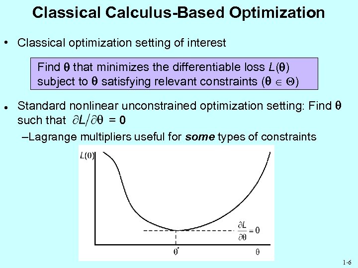Classical Calculus-Based Optimization • Classical optimization setting of interest Find that minimizes the differentiable loss L( ) subject to satisfying relevant constraints ( ) l Standard nonlinear unconstrained optimization setting: Find such that =0 –Lagrange multipliers useful for some types of constraints 1 -6

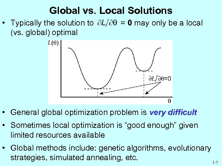Global vs. Local Solutions • Typically the solution to (vs. global) optimal = 0 may only be a local • General global optimization problem is very difficult • Sometimes local optimization is “good enough” given limited resources available • Global methods include: genetic algorithms, evolutionary strategies, simulated annealing, etc. 1 -7

Global vs. Local Solutions (cont’d) • Global methods tend to have following characteristics: – Inefficient, especially for high-dimensional – Relatively difficult to use (e. g. , require very careful selection of algorithm coefficients) – Sometimes questionable theoretical foundation for global convergence – Multiple runs usually required to have confidence in reaching global optimum • Some “hype” with many methods; e. g. , genetic algorithm (GA) software advertisement: – “…uses GAs to solve any optimization problem!” • But there are some sound methods – E. g. , restricted settings for GAs, simulated annealing, and stochastic approximation 1 -8

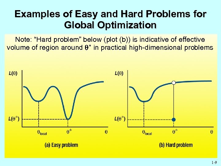Examples of Easy and Hard Problems for Global Optimization Note: “Hard problem” below (plot (b)) is indicative of effective volume of region around in practical high-dimensional problems 1 -9

Stochastic Search and Optimization • Focus here is stochastic search and optimization: A. Random noise in input information (e. g. , noisy measurements of L( ): y( ) L( ) + noise) — and/or — B. Injected randomness (Monte Carlo) in choice of algorithm iteration magnitude/direction • Contrasts with deterministic methods – E. g. , steepest descent, Newton-Raphson, etc. – Assume perfect information about L( ) (and its gradients) – Search magnitude/direction deterministic at each iteration • Injected randomness (B) in search magnitude/direction can offer benefits in efficiency and robustness – E. g. , Capabilities for global (vs. local) optimization 1 -10

Some Popular Stochastic Search and Optimization Techniques • Random search • Stochastic approximation – – – • • • Robbins-Monro and Kiefer-Wolfowitz SPSA NN backpropagation Infinitesimal perturbation analysis Recursive least squares Many others Simulated annealing Genetic algorithms Evolutionary programs and strategies Reinforcement learning Markov chain Monte Carlo (MCMC) Etc. 1 -11

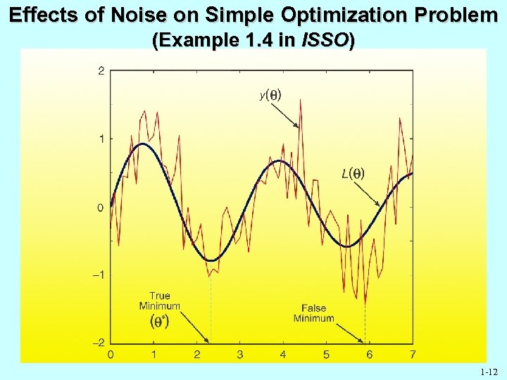Effects of Noise on Simple Optimization Problem (Example 1. 4 in ISSO) 1 -12

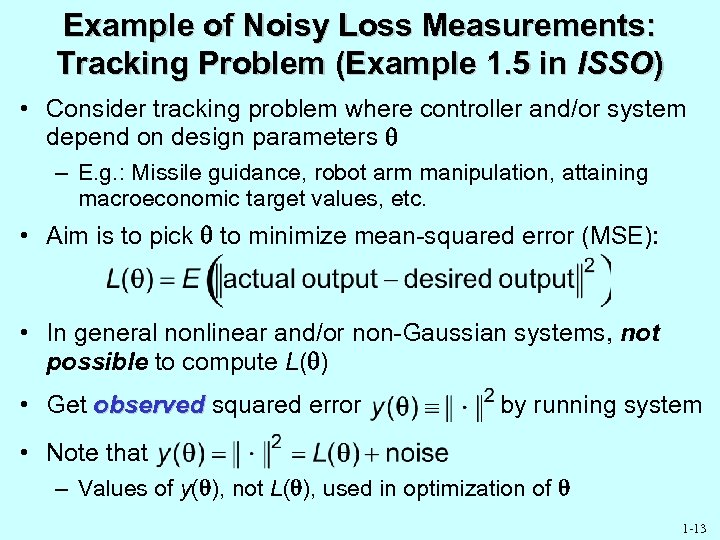Example of Noisy Loss Measurements: Tracking Problem (Example 1. 5 in ISSO) • Consider tracking problem where controller and/or system depend on design parameters – E. g. : Missile guidance, robot arm manipulation, attaining macroeconomic target values, etc. • Aim is to pick to minimize mean-squared error (MSE): • In general nonlinear and/or non-Gaussian systems, not possible to compute L( ) • Get observed squared error by running system • Note that – Values of y( ), not L( ), used in optimization of 1 -13

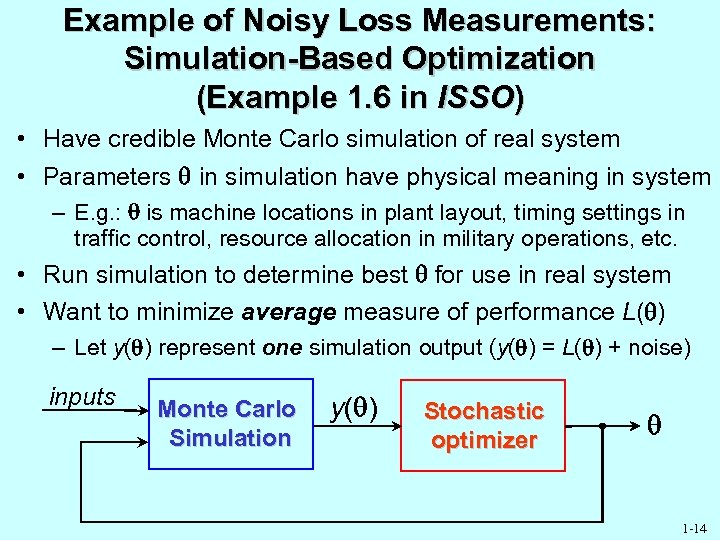Example of Noisy Loss Measurements: Simulation-Based Optimization (Example 1. 6 in ISSO) • Have credible Monte Carlo simulation of real system • Parameters in simulation have physical meaning in system – E. g. : is machine locations in plant layout, timing settings in traffic control, resource allocation in military operations, etc. • Run simulation to determine best for use in real system • Want to minimize average measure of performance L( ) – Let y( ) represent one simulation output (y( ) = L( ) + noise) inputs Monte Carlo Simulation y( ) Stochastic optimizer 1 -14

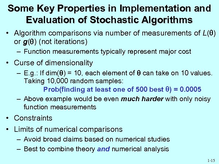Some Key Properties in Implementation and Evaluation of Stochastic Algorithms • Algorithm comparisons via number of measurements of L( ) or g( ) (not iterations) – Function measurements typically represent major cost • Curse of dimensionality – E. g. : If dim( ) = 10, each element of can take on 10 values. Taking 10, 000 random samples: Prob(finding at least one of 500 best ) = 0. 0005 – Above example would be even much harder with only noisy function measurements • Constraints • Limits of numerical comparisons – Avoid broad claims based on numerical studies – Best to combine theory and numerical analysis 1 -15

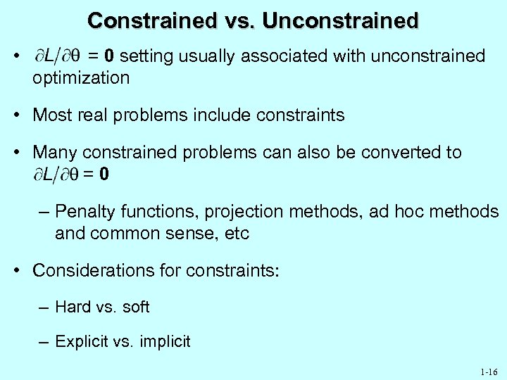Constrained vs. Unconstrained • = 0 setting usually associated with unconstrained optimization • Most real problems include constraints • Many constrained problems can also be converted to =0 – Penalty functions, projection methods, ad hoc methods and common sense, etc • Considerations for constraints: – Hard vs. soft – Explicit vs. implicit 1 -16

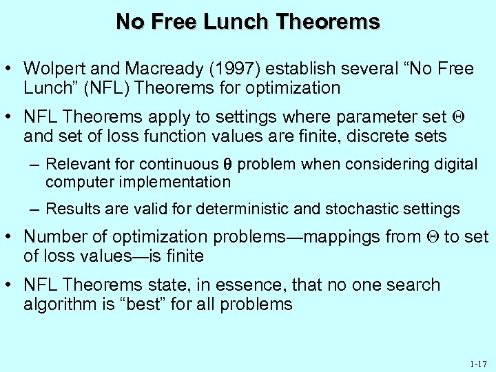No Free Lunch Theorems • Wolpert and Macready (1997) establish several “No Free Lunch” (NFL) Theorems for optimization • NFL Theorems apply to settings where parameter set and set of loss function values are finite, discrete sets – Relevant for continuous problem when considering digital computer implementation – Results are valid for deterministic and stochastic settings • Number of optimization problems—mappings from to set of loss values—is finite • NFL Theorems state, in essence, that no one search algorithm is “best” for all problems 1 -17

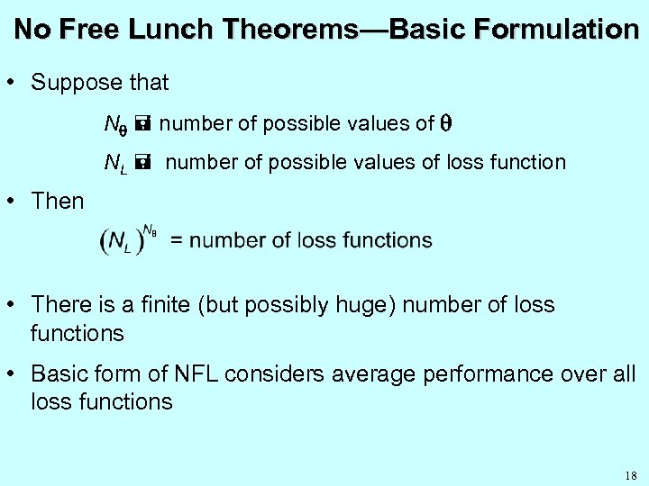No Free Lunch Theorems—Basic Formulation • Suppose that N number of possible values of NL number of possible values of loss function • There is a finite (but possibly huge) number of loss functions • Basic form of NFL considers average performance over all loss functions 18

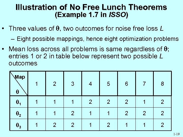Illustration of No Free Lunch Theorems (Example 1. 7 in ISSO) • Three values of , two outcomes for noise free loss L – Eight possible mappings, hence eight optimization problems • Mean loss across all problems is same regardless of ; entries 1 or 2 in table below represent two possible L outcomes Map 1 2 3 4 5 6 7 8 1 1 2 2 2 1 2 2 1 1 2 2 2 3 1 2 2 1 1 2 1 -19

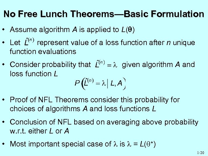No Free Lunch Theorems—Basic Formulation • Assume algorithm A is applied to L( ) • Let represent value of a loss function after n unique function evaluations • Consider probability that loss function L given algorithm A and • Proof of NFL Theorems consider this probability for choices of algorithms A and loss functions L • Conclusion of NFL based on averaging above probability w. r. t. either L or A • Most important special case of is = L( ) 1 -20

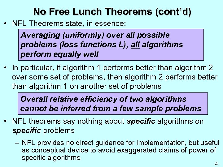No Free Lunch Theorems (cont’d) • NFL Theorems state, in essence: Averaging (uniformly) over all possible problems (loss functions L), all algorithms perform equally well • In particular, if algorithm 1 performs better than algorithm 2 over some set of problems, then algorithm 2 performs better than algorithm 1 on another set of problems Overall relative efficiency of two algorithms cannot be inferred from a few sample problems • NFL theorems say nothing about specific algorithms on specific problems – NFL provides no direct guidance for implementation, but useful as conceptual device to avoid exaggerated claims of power of specific algorithms 21

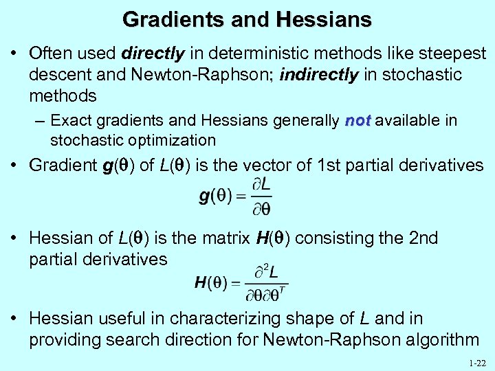Gradients and Hessians • Often used directly in deterministic methods like steepest descent and Newton-Raphson; indirectly in stochastic methods – Exact gradients and Hessians generally not available in stochastic optimization • Gradient g( ) of L( ) is the vector of 1 st partial derivatives • Hessian of L( ) is the matrix H( ) consisting the 2 nd partial derivatives • Hessian useful in characterizing shape of L and in providing search direction for Newton-Raphson algorithm 1 -22

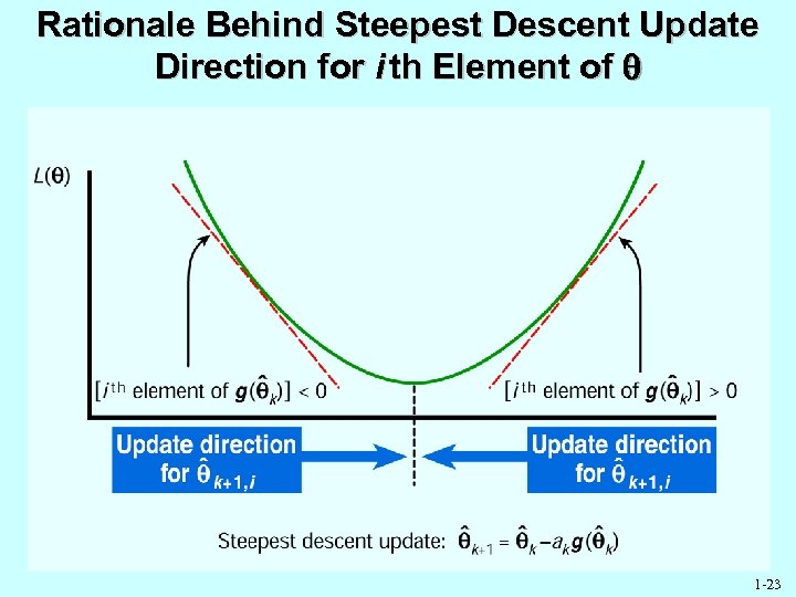Rationale Behind Steepest Descent Update Direction for i th Element of 1 -23

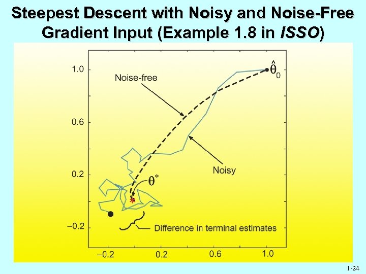Steepest Descent with Noisy and Noise-Free Gradient Input (Example 1. 8 in ISSO) 1 -24

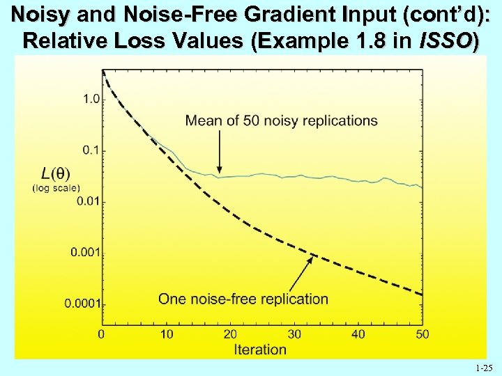Noisy and Noise-Free Gradient Input (cont’d): Relative Loss Values (Example 1. 8 in ISSO) 1 -25

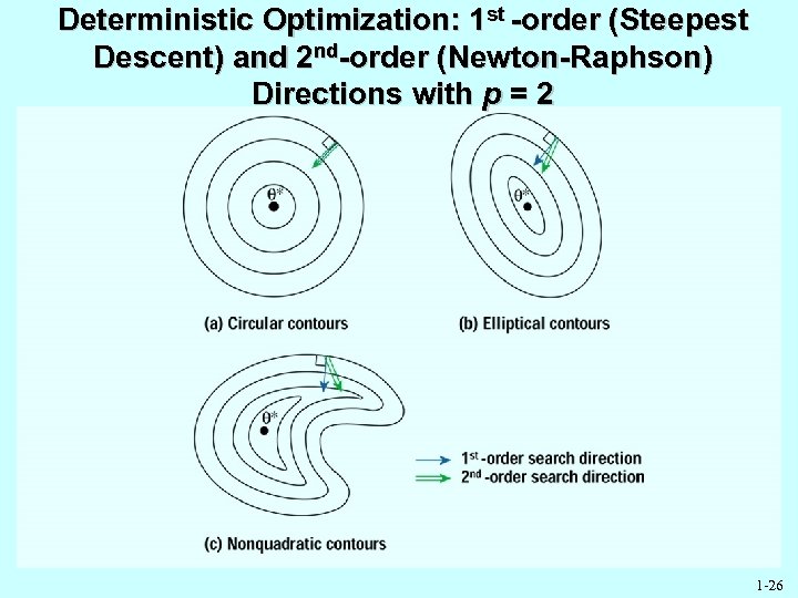Deterministic Optimization: 1 st -order (Steepest Descent) and 2 nd-order (Newton-Raphson) Directions with p = 2 1 -26

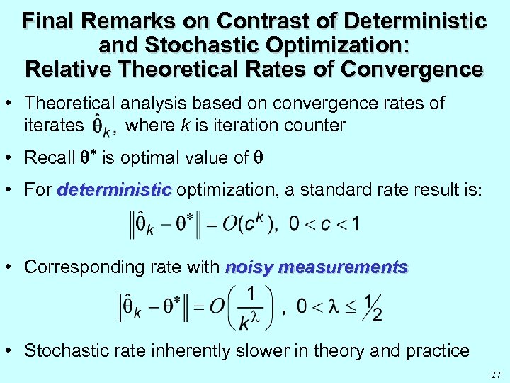Final Remarks on Contrast of Deterministic and Stochastic Optimization: Relative Theoretical Rates of Convergence • Theoretical analysis based on convergence rates of iterates where k is iteration counter • Recall is optimal value of • For deterministic optimization, a standard rate result is: • Corresponding rate with noisy measurements • Stochastic rate inherently slower in theory and practice 27

Concluding Remarks • Stochastic search and optimization very widely used – Handles noise in the function evaluations – Generally better for global optimization – Broader applicability to “non-nice” problems (robustness) • Some challenges in practical problems – – Noise dramatically affects convergence Distinguishing global from local minima not generally easy Curse of dimensionality Choosing algorithm “tuning coefficients” • Rarely sufficient to use theory for standard deterministic methods to characterize stochastic methods • “No free lunch” theorems are barrier to exaggerated claims of power and efficiency of any specific algorithm • Algorithms should be implemented in context: “Better a rough answer to the right question than an exact answer to the wrong one” (Lord Kelvin) 1 -28

Selected References on Stochastic Optimization • Fogel, D. B. (2000), Evolutionary Computation: Toward a New Philosophy of Machine Intelligence (2 nd ed. ), IEEE Press, Piscataway, NJ. • Fu, M. C. (2002), “Optimization for Simulation: Theory vs. Practice” (with discussion by S. Andradóttir, P. Glynn, and J. P. Kelly), INFORMS Journal on Computing, vol. 14, pp. 192 227. • Goldberg, D. E. (1989), Genetic Algorithms in Search, Optimization, and Machine Learning, Addison-Wesley, Reading, MA. • Gosavi, A. (2003), Simulation-Based Optimization: Parametric Optimization Techniques and Reinforcement Learning, Kluwer, Boston. • Holland, J. H. (1975), Adaptation in Natural and Artificial Systems, University of Michigan Press, Ann Arbor. • Kleijnen, J. P. C. (2008), Design and Analysis of Simulation Experiments, Springer. • Kushner, H. J. and Yin, G. G. (2003), Stochastic Approximation and Recursive Algorithms and Applications (2 nd ed. ), Springer-Verlag, New York. • Michalewicz, Z. and Fogel, D. B. (2000), How to Solve It: Modern Heuristics, Springer -Verlag, New York. • Spall, J. C. (2003), Introduction to Stochastic Search and Optimization: Estimation, Simulation, and Control, Wiley, Hoboken, NJ. • Zhigljavsky, A. A. (1991), Theory of Global Random Search, Kluwer, Boston. 29