c6b40dc7adb40484817f982d21e83386.ppt
- Количество слайдов: 35

Slides by John Loucks St. Edward’s University © 2012 Cengage Learning. All Rights Reserved. May not be scanned, copied or duplicated, or posted to a publicly accessible website, in whole or in part. Slide 1
Chapter 10, Part B Statistical Inference About Means and Proportions With Two Populations n Inferences About the Difference Between Two Population Means: Matched Samples n Inferences About the Difference Between Two Population Proportions © 2012 Cengage Learning. All Rights Reserved. May not be scanned, copied or duplicated, or posted to a publicly accessible website, in whole or in part. Slide 2
Inferences About the Difference Between Two Population Means: Matched Samples n With a matched-sample design each sampled item provides a pair of data values. n This design often leads to a smaller sampling error than the independent-sample design because variation between sampled items is eliminated as a source of sampling error. © 2012 Cengage Learning. All Rights Reserved. May not be scanned, copied or duplicated, or posted to a publicly accessible website, in whole or in part. Slide 3
Inferences About the Difference Between Two Population Means: Matched Samples n Example: Express Deliveries A Chicago-based firm has documents that must be quickly distributed to district offices throughout the U. S. The firm must decide between two delivery services, UPX (United Parcel Express) and INTEX (International Express), to transport its documents. © 2012 Cengage Learning. All Rights Reserved. May not be scanned, copied or duplicated, or posted to a publicly accessible website, in whole or in part. Slide 4
Inferences About the Difference Between Two Population Means: Matched Samples n Example: Express Deliveries In testing the delivery times of the two services, the firm sent two reports to a random sample of its district offices with one report carried by UPX and the other report carried by INTEX. Do the data on the next slide indicate a difference in mean delivery times for the two services? Use a. 05 level of significance. © 2012 Cengage Learning. All Rights Reserved. May not be scanned, copied or duplicated, or posted to a publicly accessible website, in whole or in part. Slide 5
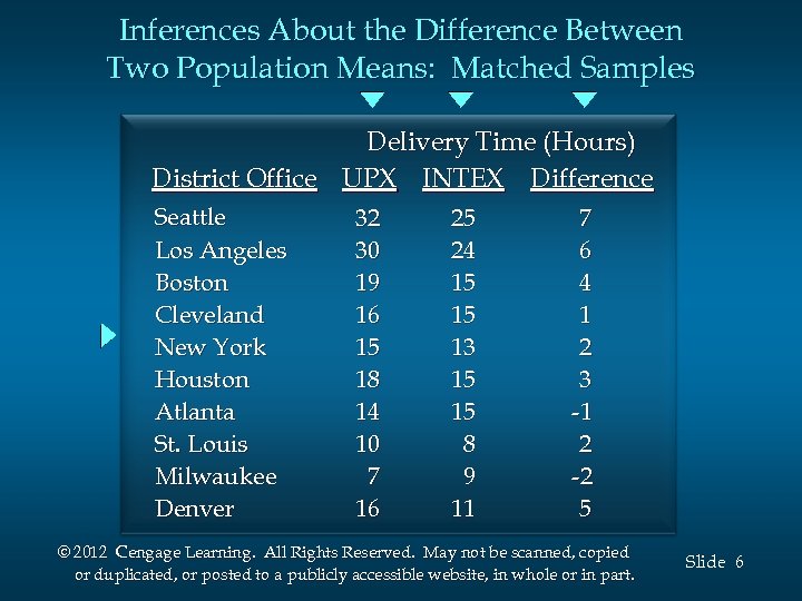
Inferences About the Difference Between Two Population Means: Matched Samples Delivery Time (Hours) District Office UPX INTEX Difference Seattle Los Angeles Boston Cleveland New York Houston Atlanta St. Louis Milwaukee Denver 32 30 19 16 15 18 14 10 7 16 25 24 15 15 13 15 15 8 9 11 7 6 4 1 2 3 -1 2 -2 5 © 2012 Cengage Learning. All Rights Reserved. May not be scanned, copied or duplicated, or posted to a publicly accessible website, in whole or in part. Slide 6
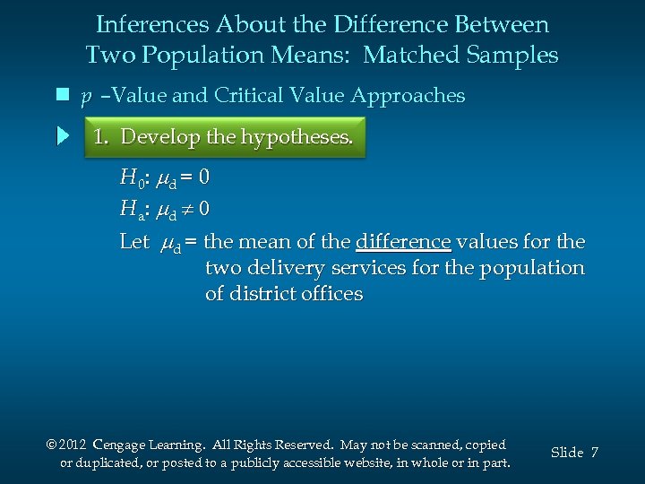
Inferences About the Difference Between Two Population Means: Matched Samples n p –Value and Critical Value Approaches 1. Develop the hypotheses. H 0: d = 0 H a: d Let d = the mean of the difference values for the two delivery services for the population of district offices © 2012 Cengage Learning. All Rights Reserved. May not be scanned, copied or duplicated, or posted to a publicly accessible website, in whole or in part. Slide 7
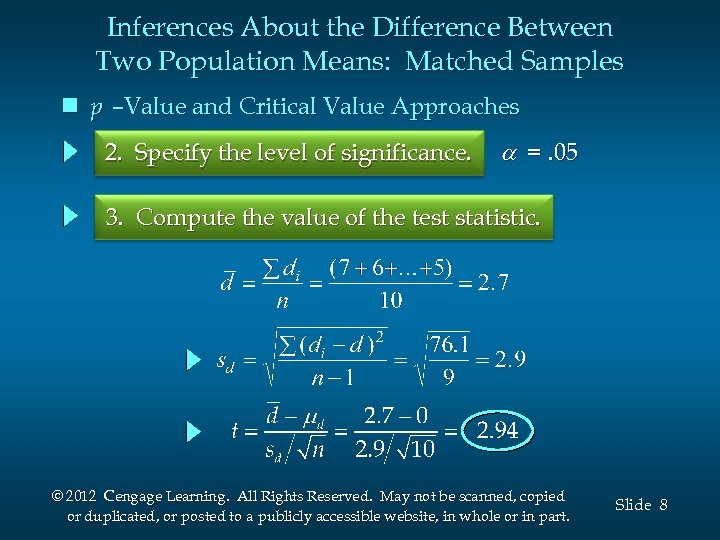
Inferences About the Difference Between Two Population Means: Matched Samples n p –Value and Critical Value Approaches 2. Specify the level of significance. =. 05 3. Compute the value of the test statistic. © 2012 Cengage Learning. All Rights Reserved. May not be scanned, copied or duplicated, or posted to a publicly accessible website, in whole or in part. Slide 8

Inferences About the Difference Between Two Population Means: Matched Samples n p –Value Approach 4. Compute the p –value. For t = 2. 94 and d. f. = 9, the p –value is between. 02 and. 01. (This is a two-tailed test, so we double the upper-tail areas of. 01 and. 005. ) 5. Determine whether to reject H 0. Because p –value < =. 05, we reject H 0. We are at least 95% confident that there is a difference in mean delivery times for the two services? © 2012 Cengage Learning. All Rights Reserved. May not be scanned, copied or duplicated, or posted to a publicly accessible website, in whole or in part. Slide 9

Inferences About the Difference Between Two Population Means: Matched Samples n Critical Value Approach 4. Determine the critical value and rejection rule. For =. 05 and d. f. = 9, t. 025 = 2. 262. Reject H 0 if t > 2. 262 5. Determine whether to reject H 0. Because t = 2. 94 > 2. 262, we reject H 0. We are at least 95% confident that there is a difference in mean delivery times for the two services? © 2012 Cengage Learning. All Rights Reserved. May not be scanned, copied or duplicated, or posted to a publicly accessible website, in whole or in part. Slide 10

Excel’s “t-Test: Paired Two Sample for Means” Tool Step 1 Click the Data tab on the Ribbon Step 2 In the Analysis group, click Data Analysis Step 3 Choose t-Test: Paired Two Sample for Means from the list of Analysis Tools Step 4 When the t-Test: Paired Two Sample for Means dialog box appears: (see details on next slide) © 2012 Cengage Learning. All Rights Reserved. May not be scanned, copied or duplicated, or posted to a publicly accessible website, in whole or in part. Slide 11
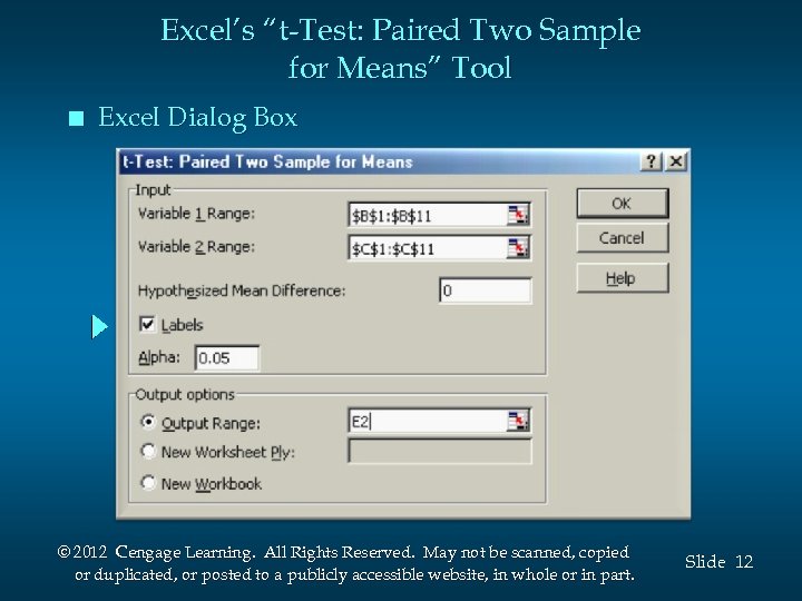
Excel’s “t-Test: Paired Two Sample for Means” Tool n Excel Dialog Box © 2012 Cengage Learning. All Rights Reserved. May not be scanned, copied or duplicated, or posted to a publicly accessible website, in whole or in part. Slide 12
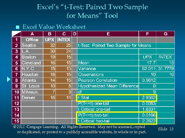
Excel’s “t-Test: Paired Two Sample for Means” Tool n Excel Value Worksheet © 2012 Cengage Learning. All Rights Reserved. May not be scanned, copied or duplicated, or posted to a publicly accessible website, in whole or in part. Slide 13
Inferences About the Difference Between Two Population Proportions n n Interval Estimation of p 1 - p 2 Hypothesis Tests About p 1 - p 2 © 2012 Cengage Learning. All Rights Reserved. May not be scanned, copied or duplicated, or posted to a publicly accessible website, in whole or in part. Slide 14
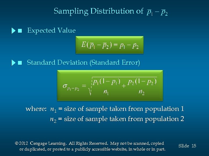
Sampling Distribution of n Expected Value n Standard Deviation (Standard Error) where: n 1 = size of sample taken from population 1 n 2 = size of sample taken from population 2 © 2012 Cengage Learning. All Rights Reserved. May not be scanned, copied or duplicated, or posted to a publicly accessible website, in whole or in part. Slide 15
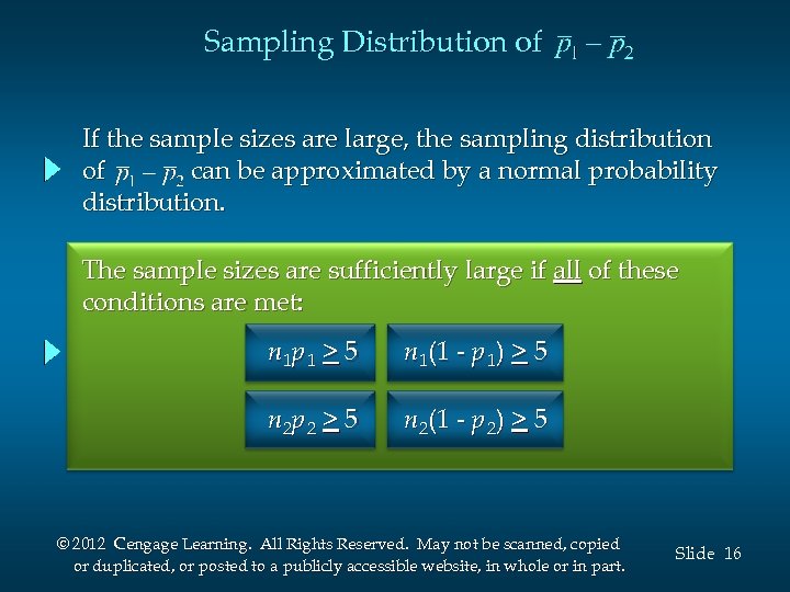
Sampling Distribution of If the sample sizes are large, the sampling distribution of can be approximated by a normal probability distribution. The sample sizes are sufficiently large if all of these conditions are met: n 1 p 1 > 5 n 1(1 - p 1) > 5 n 2 p 2 > 5 n 2(1 - p 2) > 5 © 2012 Cengage Learning. All Rights Reserved. May not be scanned, copied or duplicated, or posted to a publicly accessible website, in whole or in part. Slide 16
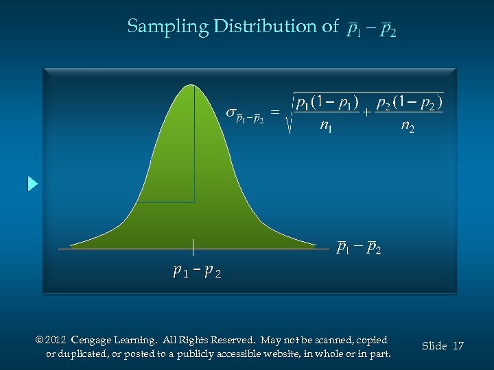
Sampling Distribution of p 1 – p 2 © 2012 Cengage Learning. All Rights Reserved. May not be scanned, copied or duplicated, or posted to a publicly accessible website, in whole or in part. Slide 17
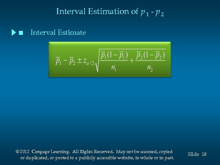
Interval Estimation of p 1 - p 2 n Interval Estimate © 2012 Cengage Learning. All Rights Reserved. May not be scanned, copied or duplicated, or posted to a publicly accessible website, in whole or in part. Slide 18

Interval Estimation of p 1 - p 2 n Example: Market Research Associates is conducting research to evaluate the effectiveness of a client’s new advertising campaign. Before the new campaign began, a telephone survey of 150 households in the test market area showed 60 households “aware” of the client’s product. The new campaign has been initiated with TV and newspaper advertisements running for three weeks. © 2012 Cengage Learning. All Rights Reserved. May not be scanned, copied or duplicated, or posted to a publicly accessible website, in whole or in part. Slide 19

Interval Estimation of p 1 - p 2 n Example: Market Research Associates A survey conducted immediately after the new campaign showed 120 of 250 households “aware” of the client’s product. Does the data support the position that the advertising campaign has provided an increased awareness of the client’s product? © 2012 Cengage Learning. All Rights Reserved. May not be scanned, copied or duplicated, or posted to a publicly accessible website, in whole or in part. Slide 20

Point Estimator of the Difference Between Two Population Proportions p 1 = proportion of the population of households “aware” of the product after the new campaign p 2 = proportion of the population of households “aware” of the product before the new campaign = sample proportion of households “aware” of the product after the new campaign = sample proportion of households “aware” of the product before the new campaign © 2012 Cengage Learning. All Rights Reserved. May not be scanned, copied or duplicated, or posted to a publicly accessible website, in whole or in part. Slide 21
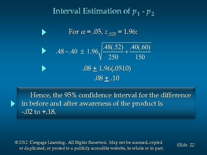
Interval Estimation of p 1 - p 2 For =. 05, z. 025 = 1. 96: . 08 + 1. 96(. 0510). 08 +. 10 Hence, the 95% confidence interval for the difference in before and after awareness of the product is -. 02 to +. 18. © 2012 Cengage Learning. All Rights Reserved. May not be scanned, copied or duplicated, or posted to a publicly accessible website, in whole or in part. Slide 22
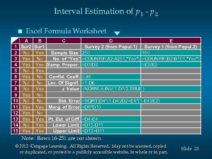
Interval Estimation of p 1 - p 2 n 1 2 3 4 5 6 7 8 9 10 11 12 13 14 15 Excel Formula Worksheet A Sur 2 No Yes No Yes Yes No Yes B Sur 1 Yes No No Yes Yes C D E Survey 2 (from Popul. 1) Survey 1 (from Popul. 2) Sample Size 250 150 No. of "Yes" =COUNTIF(A 2: A 251, "Yes") =COUNTIF(B 2: B 151, "Yes") Samp. Propor. =D 3/D 2 =E 3/E 2 Confid. Coeff. 0. 95 Lev. Of Signif. =1 -D 6 z Value =NORM. S. INV(1 -D 7/2, TRUE) Std. Error =SQRT(D 4*(1 -D 4)/D 2+E 4*(1 -E 4)/E 2) Marg. of Error =D 8*D 10 Pt. Est. of Diff. =D 4 -E 4 Lower Limit =D 13 -D 11 Upper Limit =D 13+D 11 Note: Rows 16 -251 are not shown. © 2012 Cengage Learning. All Rights Reserved. May not be scanned, copied or duplicated, or posted to a publicly accessible website, in whole or in part. Slide 23
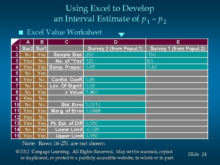
Using Excel to Develop an Interval Estimate of p 1 – p 2 n 1 2 3 4 5 6 7 8 9 10 11 12 13 14 15 Excel Value Worksheet A Sur 2 No Yes No Yes Yes No Yes B Sur 1 Yes No No Yes Yes C D E Survey 2 (from Popul. 1) Survey 1 (from Popul. 2) Sample Size 250 150 No. of "Yes" 120 60 Samp. Propor. 0. 48 0. 40 Confid. Coeff. 0. 95 Lev. Of Signif. 0. 05 z Value 1. 960 Std. Error 0. 0510 Marg. of Error 0. 0999 Pt. Est. of Diff. 0. 080 Lower Limit -0. 020 Upper Limit 0. 180 Note: Rows 16 -251 are not shown. © 2012 Cengage Learning. All Rights Reserved. May not be scanned, copied or duplicated, or posted to a publicly accessible website, in whole or in part. Slide 24
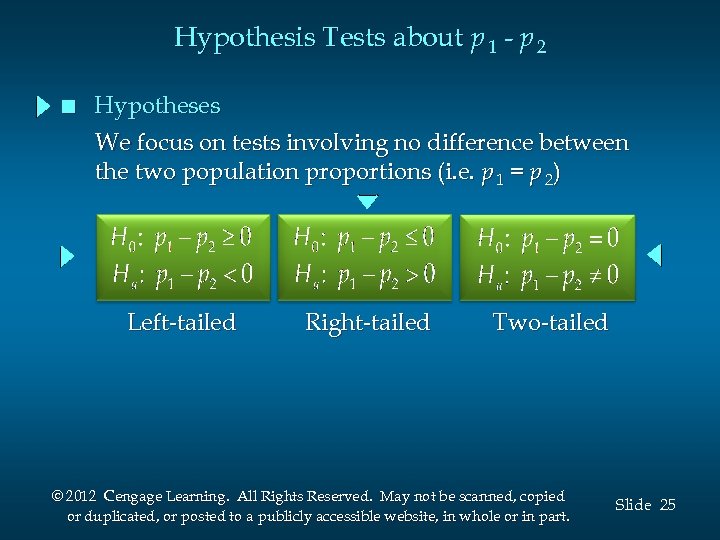
Hypothesis Tests about p 1 - p 2 n Hypotheses We focus on tests involving no difference between the two population proportions (i. e. p 1 = p 2) H 0: p 1 - p 2 < 0 H a: p 1 - p 2 > 0 Left-tailed Right-tailed Two-tailed © 2012 Cengage Learning. All Rights Reserved. May not be scanned, copied or duplicated, or posted to a publicly accessible website, in whole or in part. Slide 25
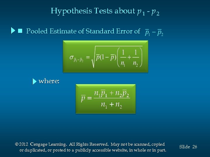
Hypothesis Tests about p 1 - p 2 n Pooled Estimate of Standard Error of where: © 2012 Cengage Learning. All Rights Reserved. May not be scanned, copied or duplicated, or posted to a publicly accessible website, in whole or in part. Slide 26
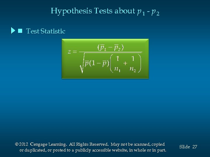
Hypothesis Tests about p 1 - p 2 n Test Statistic © 2012 Cengage Learning. All Rights Reserved. May not be scanned, copied or duplicated, or posted to a publicly accessible website, in whole or in part. Slide 27

Hypothesis Tests about p 1 - p 2 n Example: Market Research Associates Can we conclude, using a. 05 level of significance, that the proportion of households aware of the client’s product increased after the new advertising campaign? © 2012 Cengage Learning. All Rights Reserved. May not be scanned, copied or duplicated, or posted to a publicly accessible website, in whole or in part. Slide 28
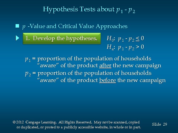
Hypothesis Tests about p 1 - p 2 n p -Value and Critical Value Approaches 1. Develop the hypotheses. H 0: p 1 - p 2 < 0 H a: p 1 - p 2 > 0 p 1 = proportion of the population of households “aware” of the product after the new campaign p 2 = proportion of the population of households “aware” of the product before the new campaign © 2012 Cengage Learning. All Rights Reserved. May not be scanned, copied or duplicated, or posted to a publicly accessible website, in whole or in part. Slide 29
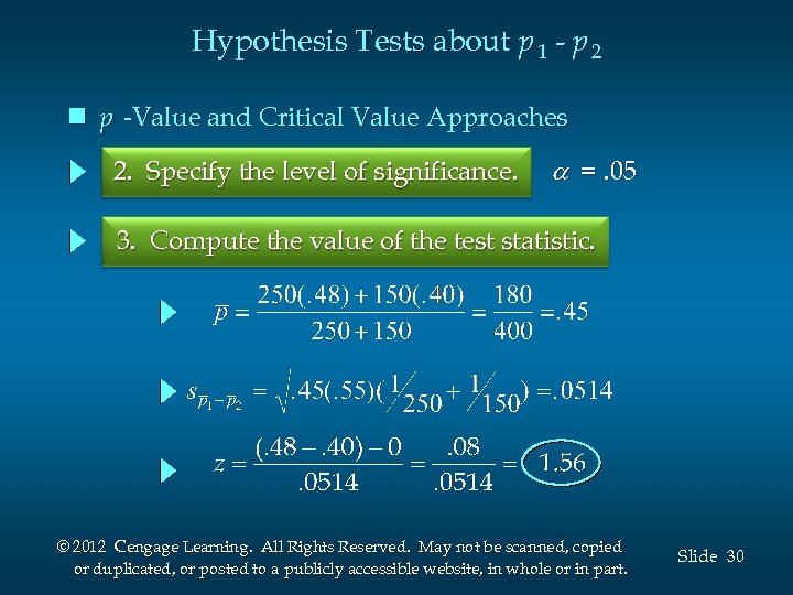
Hypothesis Tests about p 1 - p 2 n p -Value and Critical Value Approaches 2. Specify the level of significance. =. 05 3. Compute the value of the test statistic. © 2012 Cengage Learning. All Rights Reserved. May not be scanned, copied or duplicated, or posted to a publicly accessible website, in whole or in part. Slide 30

Hypothesis Tests about p 1 - p 2 n p –Value Approach 4. Compute the p –value. For z = 1. 56, the p –value =. 0594 5. Determine whether to reject H 0. Because p –value > =. 05, we cannot reject H 0. We cannot conclude that the proportion of households aware of the client’s product increased after the new campaign. © 2012 Cengage Learning. All Rights Reserved. May not be scanned, copied or duplicated, or posted to a publicly accessible website, in whole or in part. Slide 31
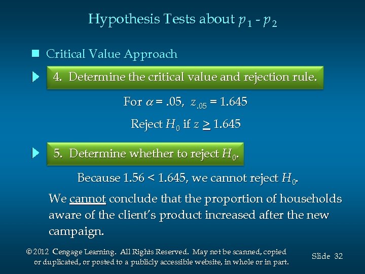
Hypothesis Tests about p 1 - p 2 n Critical Value Approach 4. Determine the critical value and rejection rule. For =. 05, z. 05 = 1. 645 Reject H 0 if z > 1. 645 5. Determine whether to reject H 0. Because 1. 56 < 1. 645, we cannot reject H 0. We cannot conclude that the proportion of households aware of the client’s product increased after the new campaign. © 2012 Cengage Learning. All Rights Reserved. May not be scanned, copied or duplicated, or posted to a publicly accessible website, in whole or in part. Slide 32
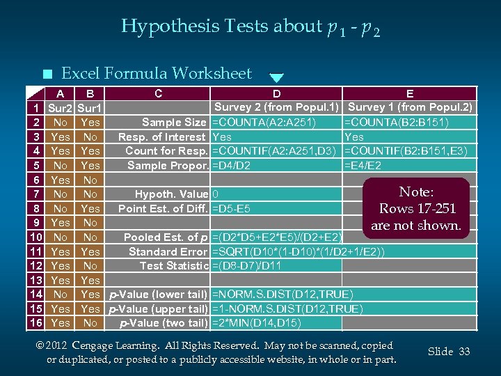
Hypothesis Tests about p 1 - p 2 n 1 2 3 4 5 6 7 8 9 10 11 12 13 14 15 16 Excel Formula Worksheet A Sur 2 No Yes No Yes Yes No Yes B C D E Survey 2 (from Popul. 1) Survey 1 (from Popul. 2) Sur 1 Yes Sample Size =COUNTA(A 2: A 251) =COUNTA(B 2: B 151) No Resp. of Interest Yes Yes Count for Resp. =COUNTIF(A 2: A 251, D 3) =COUNTIF(B 2: B 151, E 3) Yes Sample Propor. =D 4/D 2 =E 4/E 2 No Note: No Hypoth. Value 0 Yes Point Est. of Diff. =D 5 -E 5 Rows 17 -251 No are not shown. No Pooled Est. of p =(D 2*D 5+E 2*E 5)/(D 2+E 2) Yes Standard Error =SQRT(D 10*(1 -D 10)*(1/D 2+1/E 2)) No Test Statistic =(D 8 -D 7)/D 11 Yes p-Value (lower tail) =NORM. S. DIST(D 12, TRUE) Yes p-Value (upper tail) =1 -NORM. S. DIST(D 12, TRUE) No p-Value (two tail) =2*MIN(D 14, D 15) © 2012 Cengage Learning. All Rights Reserved. May not be scanned, copied or duplicated, or posted to a publicly accessible website, in whole or in part. Slide 33
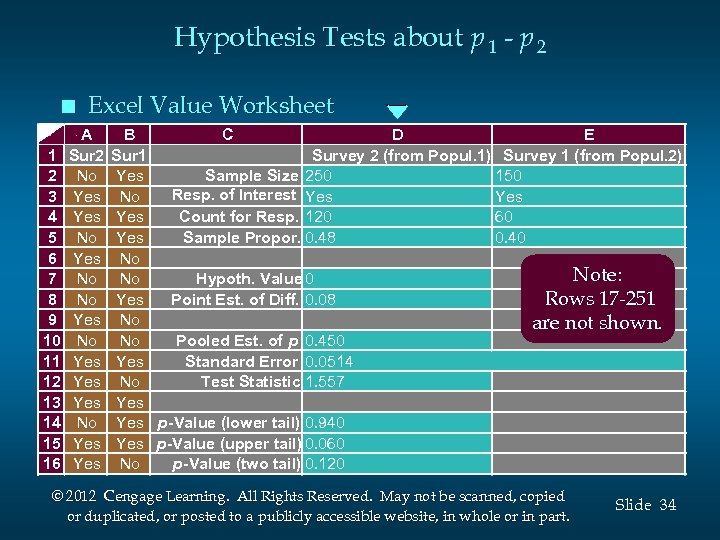
Hypothesis Tests about p 1 - p 2 n 1 2 3 4 5 6 7 8 9 10 11 12 13 14 15 16 Excel Value Worksheet A Sur 2 No Yes No Yes Yes No Yes B C D E Sur 1 Survey 2 (from Popul. 1) Survey 1 (from Popul. 2) Yes Sample Size 250 150 Resp. of Interest Yes No Yes Count for Resp. 120 60 Yes Sample Propor. 0. 48 0. 40 No Note: No Hypoth. Value 0 Yes Point Est. of Diff. 0. 08 Rows 17 -251 No are not shown. No Pooled Est. of p 0. 450 Yes Standard Error 0. 0514 No Test Statistic 1. 557 Yes p -Value (lower tail) 0. 940 Yes p -Value (upper tail) 0. 060 No p -Value (two tail) 0. 120 © 2012 Cengage Learning. All Rights Reserved. May not be scanned, copied or duplicated, or posted to a publicly accessible website, in whole or in part. Slide 34
End of Chapter 10, Part B © 2012 Cengage Learning. All Rights Reserved. May not be scanned, copied or duplicated, or posted to a publicly accessible website, in whole or in part. Slide 35
c6b40dc7adb40484817f982d21e83386.ppt