Simple Linear Regression Least squares procedure Inference for

Simple Linear Regression Least squares procedure Inference for least squares lines 1

Introduction • We will examine the relationship between quantitative variables x and y via a mathematical equation. • The motivation for using the technique: – Forecast the value of a dependent variable (y) from the value of independent variables (x 1, x 2, …xk. ). – Analyze the specific relationships between the independent variables and the 2 dependent variable.

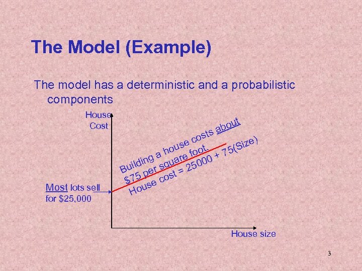The Model (Example) The model has a deterministic and a probabilistic components House Cost Most lots sell for $25, 000 out ab s ost c ize) se t. (S ou a h re foo 0 + 75 g ldin r squa 2500 Bui pe t= 75 e cos $ ous H House size 3

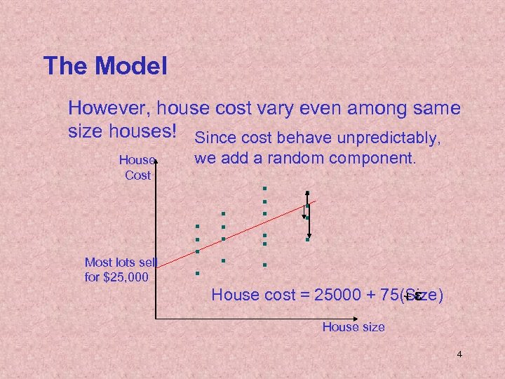The Model However, house cost vary even among same size houses! Since cost behave unpredictably, House Cost Most lots sell for $25, 000 we add a random component. +e House cost = 25000 + 75(Size) House size 4

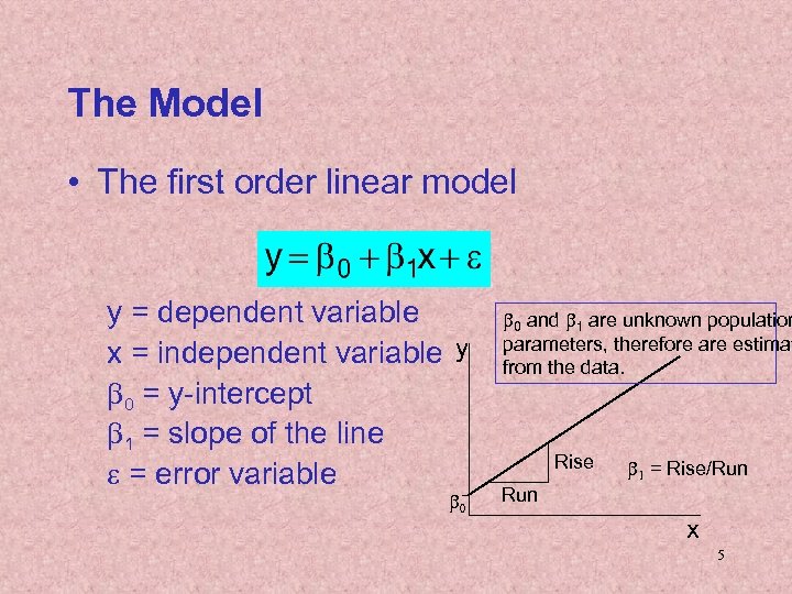The Model • The first order linear model y = dependent variable x = independent variable y b 0 = y-intercept b 1 = slope of the line e = error variable b 0 and b 1 are unknown population parameters, therefore are estimat from the data. Rise b 1 = Rise/Run x 5

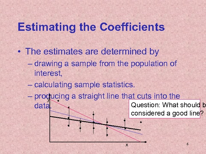Estimating the Coefficients • The estimates are determined by – drawing a sample from the population of interest, – calculating sample statistics. – producing a straight line that cuts into the y w Question: What should b data. w w w considered a good line? w w w x 6

The Least Squares (Regression) Line A good line is one that minimizes the sum of squared differences between the points and the line. 7

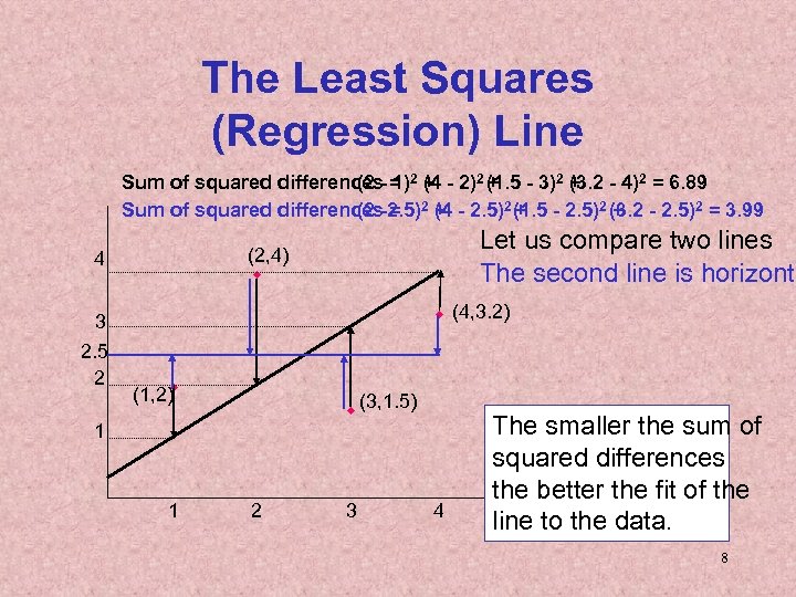The Least Squares (Regression) Line Sum of squared differences- = 2 + - 2)2 (1. 5 - 3)2 + - 4)2 = 6. 89 (2 1) (4 + (3. 2 Sum of squared differences-2. 5)2 + - 2. 5)2 (1. 5 - 2. 5)2 (3. 2 - 2. 5)2 = 3. 99 (2 = (4 + + 3 2. 5 2 Let us compare two lines The second line is horizonta (2, 4) w 4 w (4, 3. 2) w (1, 2) w (3, 1. 5) 1 1 2 3 4 The smaller the sum of squared differences the better the fit of the line to the data. 8

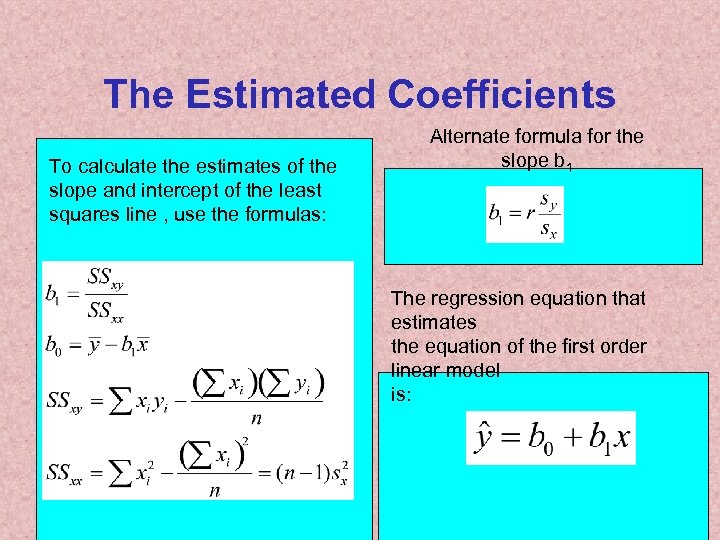The Estimated Coefficients To calculate the estimates of the slope and intercept of the least squares line , use the formulas: Alternate formula for the slope b 1 The regression equation that estimates the equation of the first order linear model is: 9

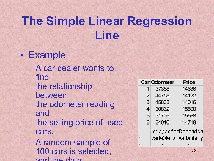The Simple Linear Regression Line • Example: – A car dealer wants to find the relationship between the odometer reading and the selling price of used cars. – A random sample of 100 cars is selected, Independent Dependent variable x variable y 10

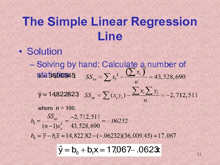The Simple Linear Regression Line • Solution – Solving by hand: Calculate a number of statistics where n = 100. 11

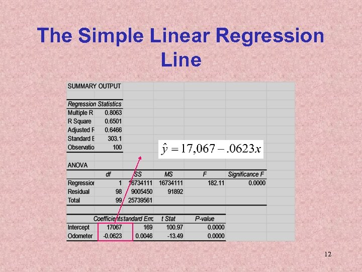The Simple Linear Regression Line 12

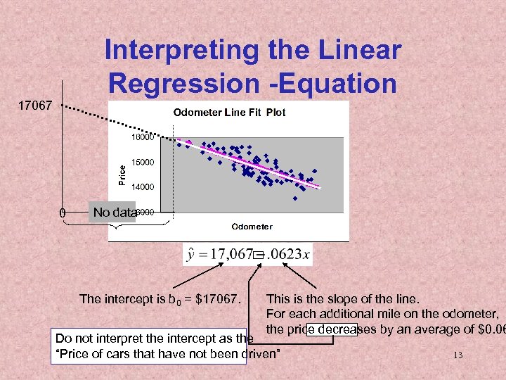Interpreting the Linear Regression -Equation 17067 0 No data The intercept is b 0 = $17067. This is the slope of the line. For each additional mile on the odometer, the price decreases by an average of $0. 06 Do not interpret the intercept as the “Price of cars that have not been driven” 13

Error Variable: Required Conditions • The error e is a critical part of the regression model. • Four requirements involving the distribution of e must be satisfied. – The probability distribution of e is normal. – The mean of e is zero: E(e) = 0. – The standard deviation of e is se for all values of x. – The set of errors associated with different 14

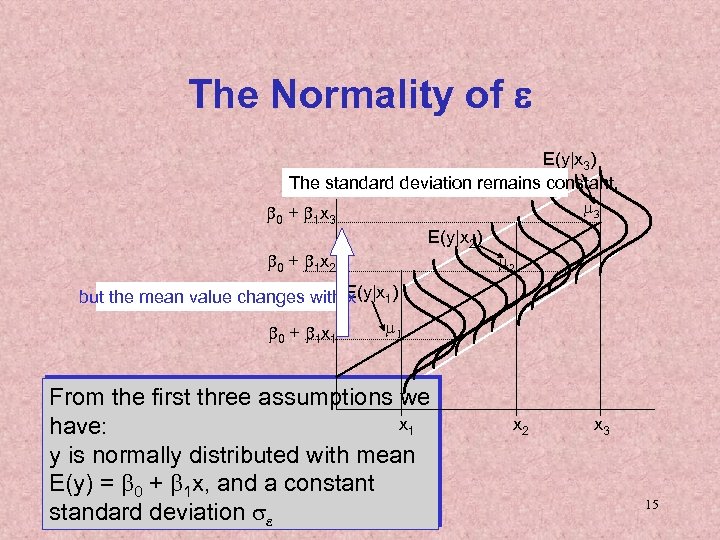The Normality of e E(y|x 3) The standard deviation remains constant, m 3 b 0 + b 1 x 3 E(y|x 2) b 0 + b 1 x 2 m 2 but the mean value changes with E(y|x 1) x b 0 + b 1 x 1 m 1 From the first three assumptions we x 1 have: y is normally distributed with mean E(y) = b 0 + b 1 x, and a constant standard deviation se x 2 x 3 15

Assessing the Model • The least squares method will produces a regression line whether or not there is a linear relationship between x and y. • Consequently, it is important to assess how well the linear model fits the data. • Several methods are used to assess the model. All are based on the sum of squares for errors, SSE. 16

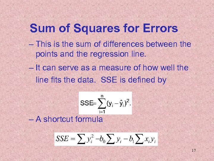Sum of Squares for Errors – This is the sum of differences between the points and the regression line. – It can serve as a measure of how well the line fits the data. SSE is defined by – A shortcut formula 17

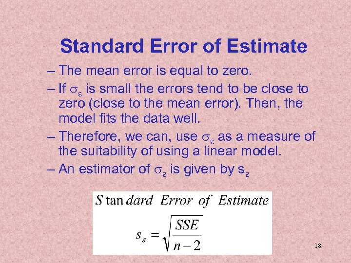Standard Error of Estimate – The mean error is equal to zero. – If se is small the errors tend to be close to zero (close to the mean error). Then, the model fits the data well. – Therefore, we can, use se as a measure of the suitability of using a linear model. – An estimator of se is given by se 18

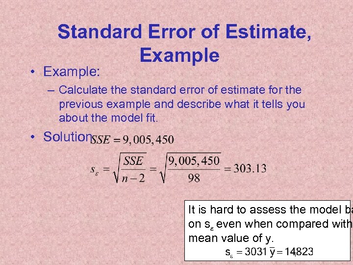Standard Error of Estimate, Example • Example: – Calculate the standard error of estimate for the previous example and describe what it tells you about the model fit. • Solution It is hard to assess the model ba on se even when compared with mean value of y. 19

“p-values” and Significance Levels Each independent variable has “p-value” or significance level. The p-value tells how likely it is that the coefficient for that independent variable emerged by chance and does not describe a real relationship. A p-value of. 05 means that there is a 5% chance that the relationship emerged randomly and a 95% chance that the relationship is real. It is generally accepted practice to consider variables with a p-value of less than. 1 as significant, though the only basis for this cutoff 20 is

Using the Regression Equation • Before using the regression model, we need to assess how well it fits the data. • If we are satisfied with how well the model fits the data, we can use it to predict the values of y. • To make a prediction we use – Point prediction, and – Interval prediction 21

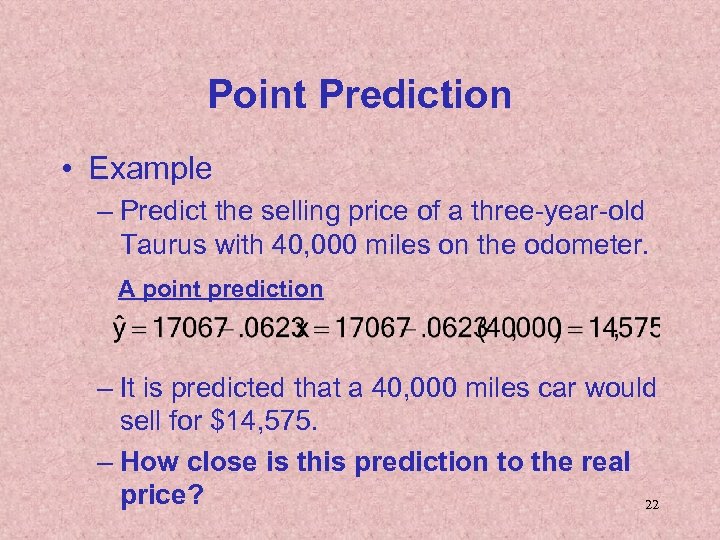Point Prediction • Example – Predict the selling price of a three-year-old Taurus with 40, 000 miles on the odometer. A point prediction – It is predicted that a 40, 000 miles car would sell for $14, 575. – How close is this prediction to the real price? 22

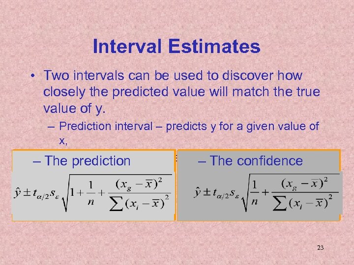Interval Estimates • Two intervals can be used to discover how closely the predicted value will match the true value of y. – Prediction interval – predicts y for a given value of x, – Confidence interval – estimates the average y for a – The prediction – The confidence given x. interval 23

Interval Estimates, Example • Example - continued – Provide an interval estimate for the bidding price on a Ford Taurus with 40, 000 miles on the odometer. – Two types of predictions are required: • A prediction for a specific car • An estimate for the average price per car 24

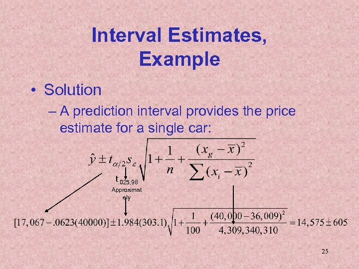Interval Estimates, Example • Solution – A prediction interval provides the price estimate for a single car: t. 025, 98 Approximat ely 25

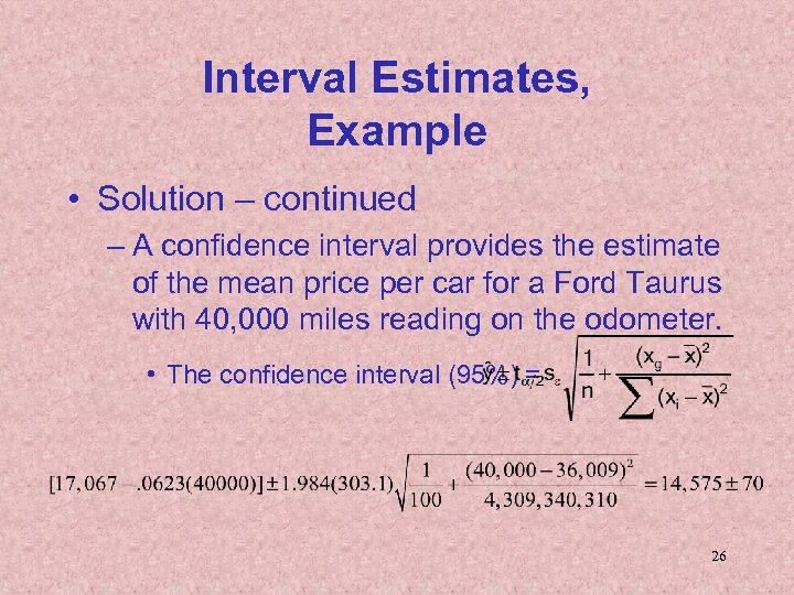Interval Estimates, Example • Solution – continued – A confidence interval provides the estimate of the mean price per car for a Ford Taurus with 40, 000 miles reading on the odometer. • The confidence interval (95%) = 26

Residual Analysis • Examining the residuals (or standardized residuals), help detect violations of the required conditions. • Example – continued: – Nonnormality. • Use Excel to obtain the standardized residual histogram. • Examine the histogram and look for a bell shaped. diagram with a mean close to zero. 27

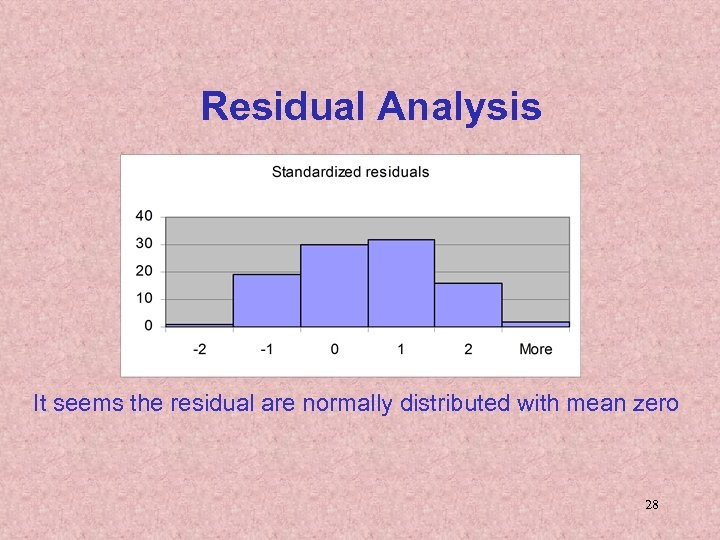Residual Analysis It seems the residual are normally distributed with mean zero 28

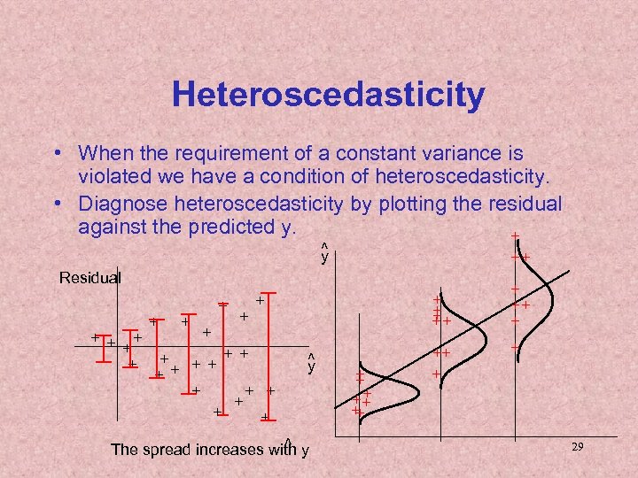Heteroscedasticity • When the requirement of a constant variance is violated we have a condition of heteroscedasticity. • Diagnose heteroscedasticity by plotting the residual against the predicted y. + ^ y ++ Residual + + + ++ + + + ^ y ^ The spread increases with y + ++ + + 29

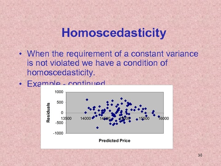Homoscedasticity • When the requirement of a constant variance is not violated we have a condition of homoscedasticity. • Example - continued 30

Non Independence of Error Variables – A time series is constituted if data were collected over time. – Examining the residuals over time, no pattern should be observed if the errors are independent. – When a pattern is detected, the errors are said to be autocorrelated. – Autocorrelation can be detected by graphing the residuals against time. 31

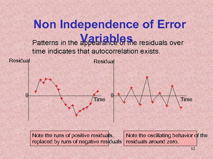Non Independence of Error Variables Patterns in the appearance of the residuals over time indicates that autocorrelation exists. Residual + ++ + 0 + + ++ + 0 + Time + + Note the runs of positive residuals, Note the oscillating behavior of the replaced by runs of negative residuals around zero. 32

Outliers • An outlier is an observation that is unusually small or large. • Several possibilities need to be investigated when an outlier is observed: – There was an error in recording the value. – The point does not belong in the sample. – The observation is valid. • Identify outliers from the scatter diagram. • It is customary to suspect an observation is an outlier if its |standard residual| > 2 33

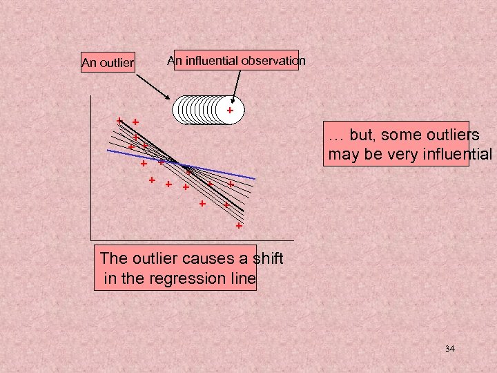An outlier An influential observation + + + + +++++ … but, some outliers may be very influential + + + + The outlier causes a shift in the regression line 34

Procedure for Regression Diagnostics • Develop a model that has a theoretical basis. • Gather data for the two variables in the model. • Draw the scatter diagram to determine whether a linear model appears to be appropriate. • Determine the regression equation. • Check the required conditions for the errors. • Check the existence of outliers and influential observations • Assess the model fit. • If the model fits the data, use the regression equation. 35