SIAM Imaging Science July 2008 Discriminative Approach

SIAM – Imaging Science, July 2008 Discriminative Approach for Transform Based Image Restoration Yacov Hel-Or Doron Shaked Gil Ben-Artzi The Interdisciplinary Center Israel HP Las Bar-Ilan Univ. Israel

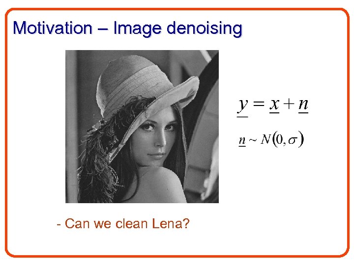Motivation – Image denoising - Can we clean Lena?

Broader Scope • • Inpainting De-blurring De-noising De-mosaicing • All the above deal with degraded images. • Their reconstruction requires solving an inverse problem

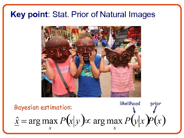Key point: Stat. Prior of Natural Images Bayesian estimation: likelihood prior

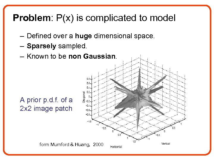Problem: P(x) is complicated to model – Defined over a huge dimensional space. – Sparsely sampled. – Known to be non Gaussian. A prior p. d. f. of a 2 x 2 image patch form Mumford & Huang, 2000

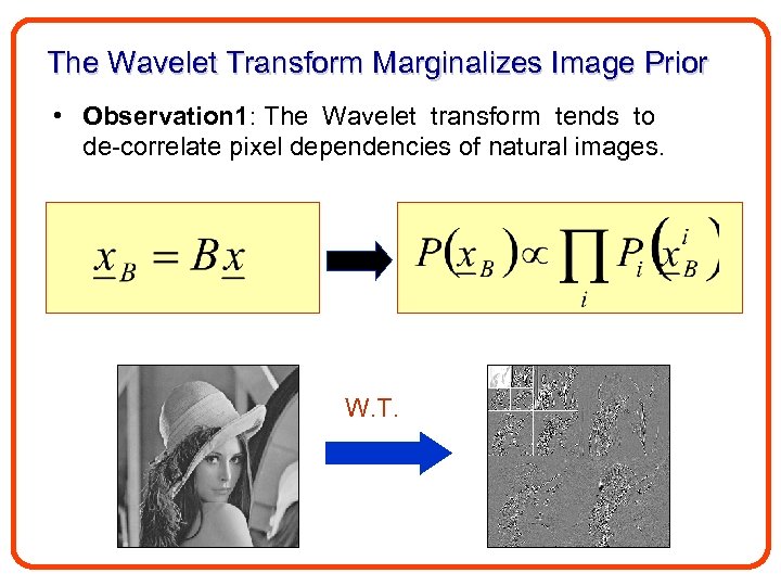The Wavelet Transform Marginalizes Image Prior • Observation 1: The Wavelet transform tends to de-correlate pixel dependencies of natural images. W. T.

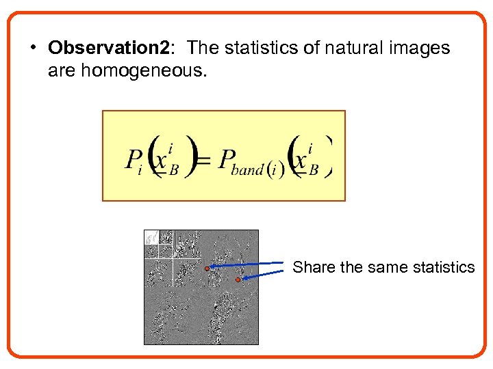• Observation 2: The statistics of natural images are homogeneous. Share the same statistics

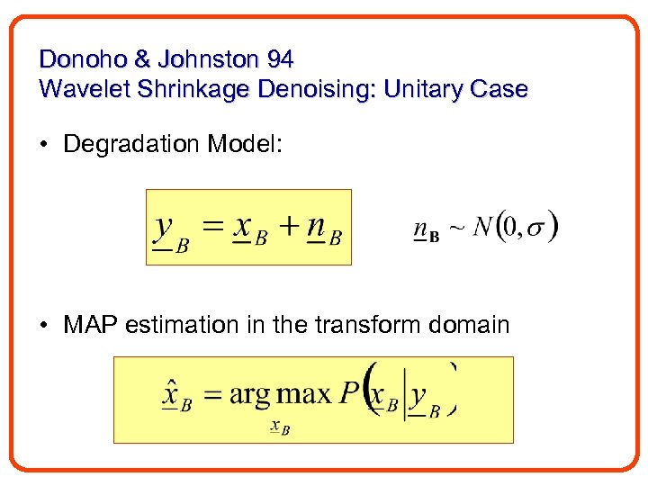Donoho & Johnston 94 Wavelet Shrinkage Denoising: Unitary Case • Degradation Model: • MAP estimation in the transform domain

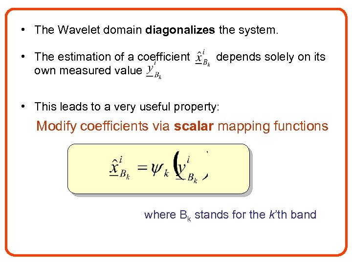• The Wavelet domain diagonalizes the system. • The estimation of a coefficient own measured value depends solely on its • This leads to a very useful property: Modify coefficients via scalar mapping functions where Bk stands for the k’th band

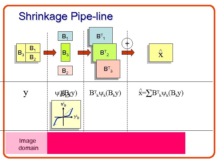Shrinkage Pipe-line B 1 B 3 y B 2 BT 1 B 3 x BT 2 BT 3 B 2 y + k(Bky) Bky BTk k(Bky) x= BTk k(Bky) xi. B yi. B Image domain Transform domain Image domain Result

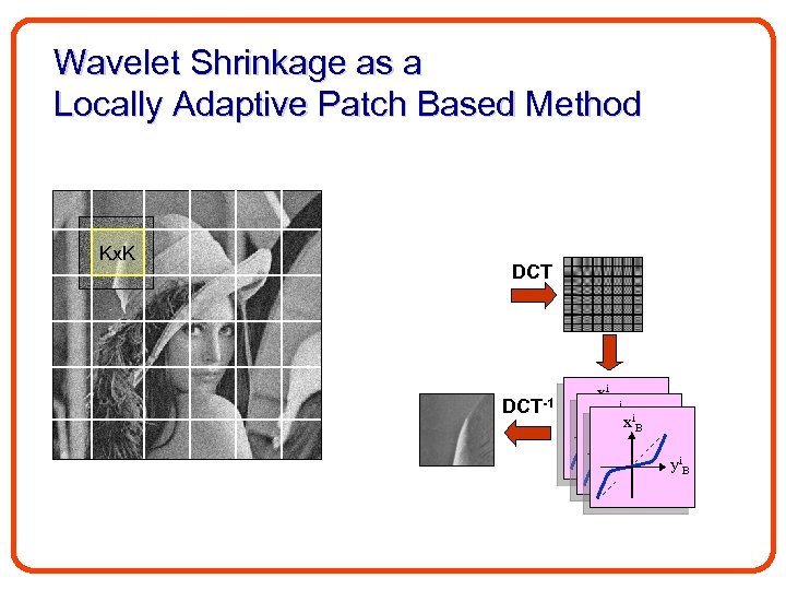Wavelet Shrinkage as a Locally Adaptive Patch Based Method Kx. K DCT-1 xi. B i x. B yi. B i y. B

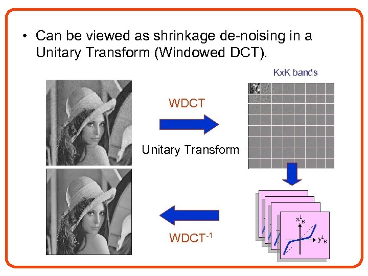• Can be viewed as shrinkage de-noising in a Unitary Transform (Windowed DCT). Kx. K bands WDCT Unitary Transform xi. B WDCT-1 yi. B

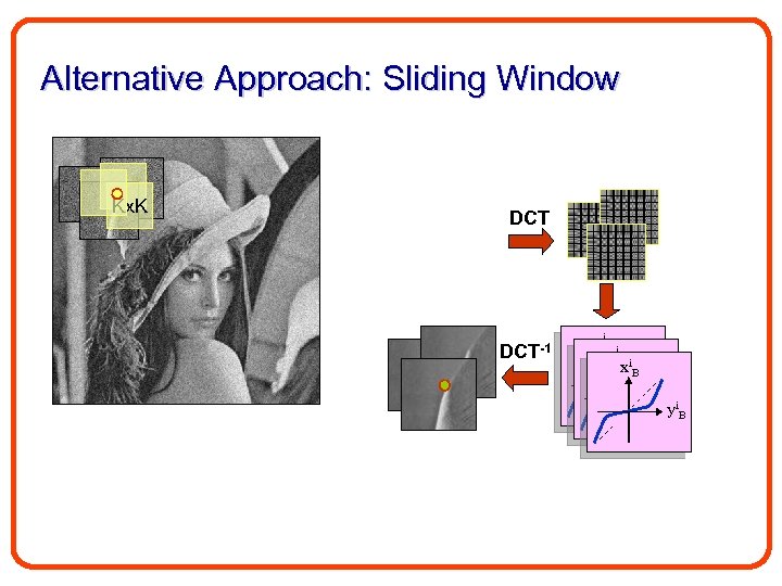Alternative Approach: Sliding Window Kx. K DCT-1 xi. B i x Bi x. B yi. B i y Bi y. B

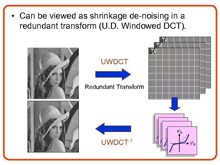• Can be viewed as shrinkage de-noising in a redundant transform (U. D. Windowed DCT). UWDCT Redundant Transform xi. B UWDCT-1 yi. B

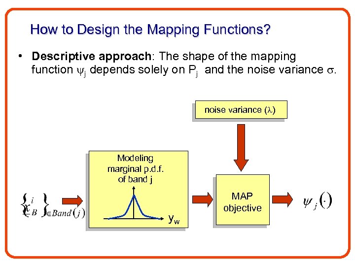How to Design the Mapping Functions? • Descriptive approach: The shape of the mapping function j depends solely on Pj and the noise variance ( ) Modeling marginal p. d. f. of band j yw MAP objective

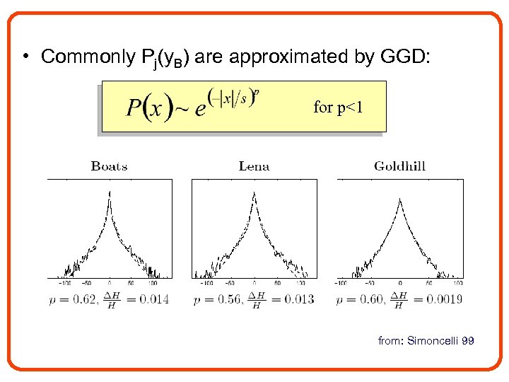• Commonly Pj(y. B) are approximated by GGD: for p<1 from: Simoncelli 99

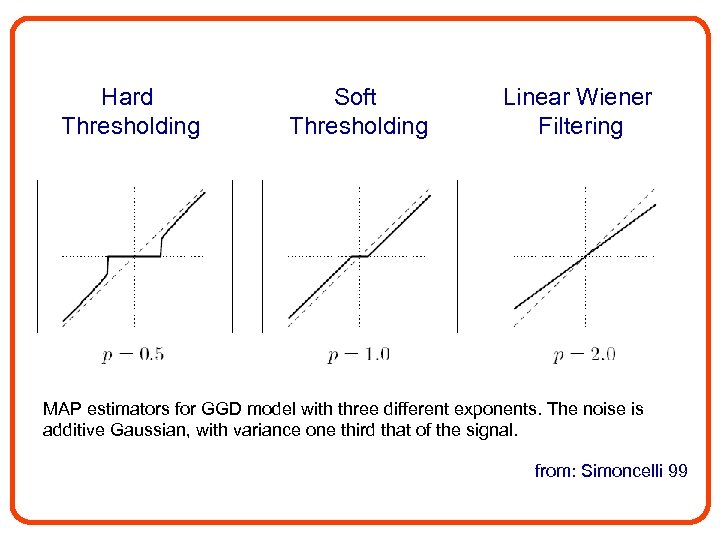Hard Thresholding Soft Thresholding Linear Wiener Filtering MAP estimators for GGD model with three different exponents. The noise is additive Gaussian, with variance one third that of the signal. from: Simoncelli 99

• Due to its simplicity Wavelet Shrinkage became extremely popular: – Thousands of applications. – Thousands of related papers • What about efficiency? – Denoising performance of the original Wavelet Shrinkage technique is far from the state-of-the-art results. • Why? – Wavelet coefficients are not really independent.

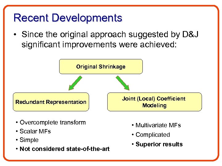Recent Developments • Since the original approach suggested by D&J significant improvements were achieved: Original Shrinkage Redundant Representation • Overcomplete transform • Scalar MFs • Simple • Not considered state-of-the-art Joint (Local) Coefficient Modeling • Multivariate MFs • Complicated • Superior results

What’s wrong with existing redundant Shrinkage? 1. Mapping functions: – Naively borrowed from the unitary case. 2. Independence assumption: – In the overcomplete case, the wavelet coefficients are inherently dependent. 3. Minimization domain: – For the unitary case MFs are optimized in the transform domain. This is incorrect in the overcomplete case (Parseval is not valid anymore). 4. Unsubstantiated – Improvements are shown empirically.

Questions we are going to address • How to design optimal MFs for redundant bases. • What is the role of redundancy. • What is the role of the domain in which the MFs are optimized. • We show that the shrinkage approach is comparable to state-of-the-art approaches where MFs are correctly designed.

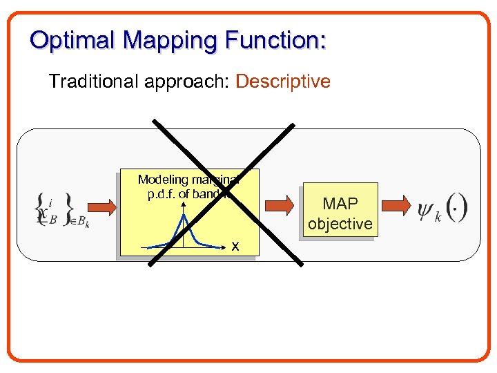Optimal Mapping Function: Traditional approach: Descriptive Modeling marginal p. d. f. of band k x MAP objective

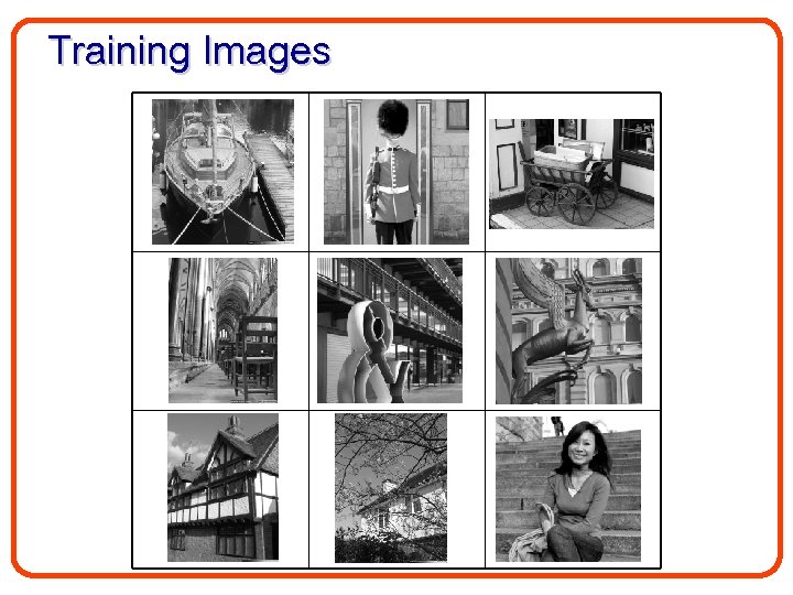
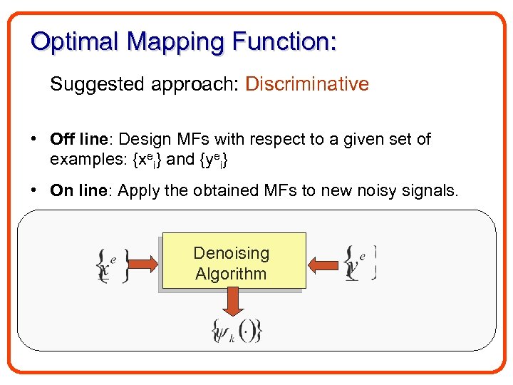Optimal Mapping Function: Suggested approach: Discriminative • Off line: Design MFs with respect to a given set of examples: {xei} and {yei} • On line: Apply the obtained MFs to new noisy signals. Denoising Algorithm

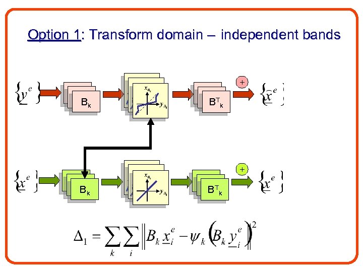Option 1: Transform domain – independent bands + B 1 B 1 Bk B 1 B 1 T B k

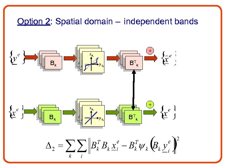Option 2: Spatial domain – independent bands + B 1 B 1 Bk B 1 B 1 T B k

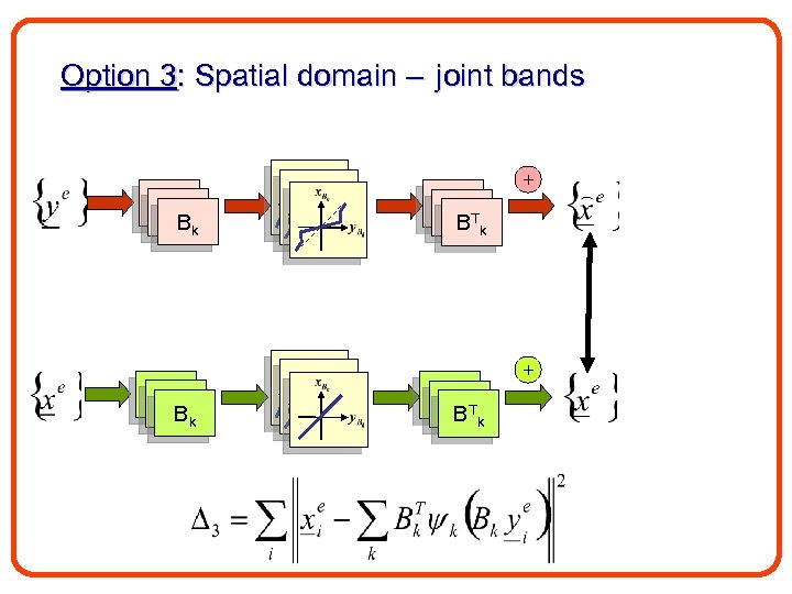Option 3: Spatial domain – joint bands + B 1 B 1 Bk B 1 B 1 T B k

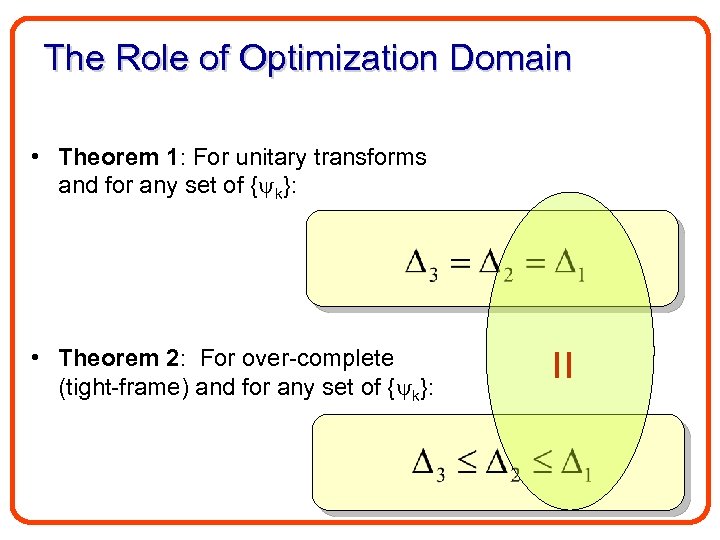The Role of Optimization Domain • Theorem 1: For unitary transforms and for any set of { k}: = • Theorem 2: For over-complete (tight-frame) and for any set of { k}:

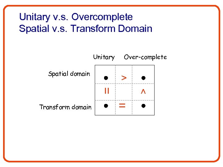Unitary v. s. Overcomplete Spatial v. s. Transform Domain Unitary Spatial domain Over-complete > > = Transform domain =

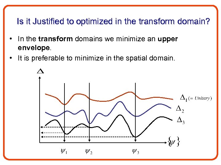Is it Justified to optimized in the transform domain? • In the transform domains we minimize an upper envelope. • It is preferable to minimize in the spatial domain.

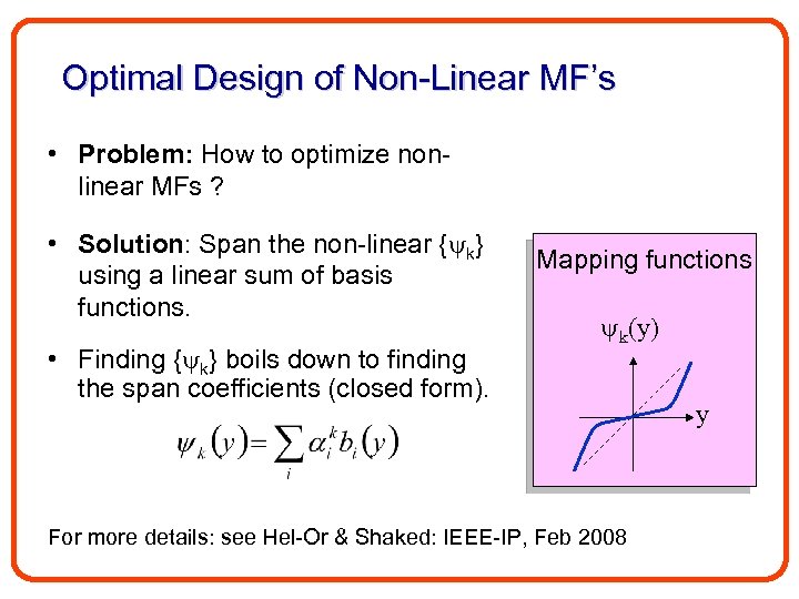Optimal Design of Non-Linear MF’s • Problem: How to optimize nonlinear MFs ? • Solution: Span the non-linear { k} using a linear sum of basis functions. • Finding { k} boils down to finding the span coefficients (closed form). Mapping functions k(y) For more details: see Hel-Or & Shaked: IEEE-IP, Feb 2008 y

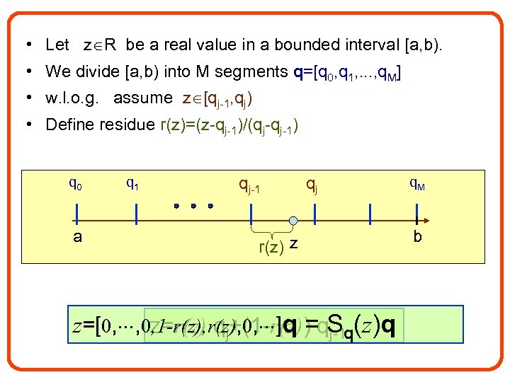• Let z R be a real value in a bounded interval [a, b). • We divide [a, b) into M segments q=[q 0, q 1, . . . , q. M] • w. l. o. g. assume z [qj-1, qj) • Define residue r(z)=(z-qj-1)/(qj-qj-1) q 0 a q 1 qj-1 qj r(z) z z=[0, , 0 z=r(z), 0, ]q =q. Sq(z)q , 1 -r(z), qj+(1 -r(z)) j-1 q. M b

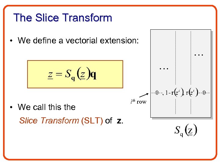The Slice Transform • We define a vectorial extension: • We call this the Slice Transform (SLT) of z. ith row

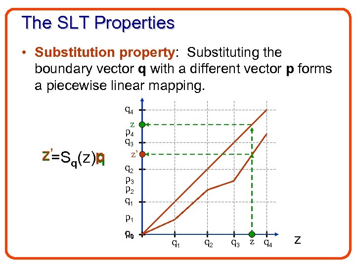The SLT Properties • Substitution property: Substituting the boundary vector q with a different vector p forms a piecewise linear mapping. q 4 z z’=Sq(z)p q p 4 q 3 z’ q 2 p 3 p 2 q 1 p 1 q 0 p q 1 q 2 q 3 z q 4 z

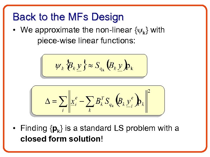Back to the MFs Design • We approximate the non-linear { k} with piece-wise linear functions: • Finding {pk} is a standard LS problem with a closed form solution!

Results

Training Images

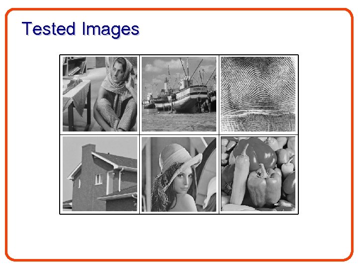Tested Images

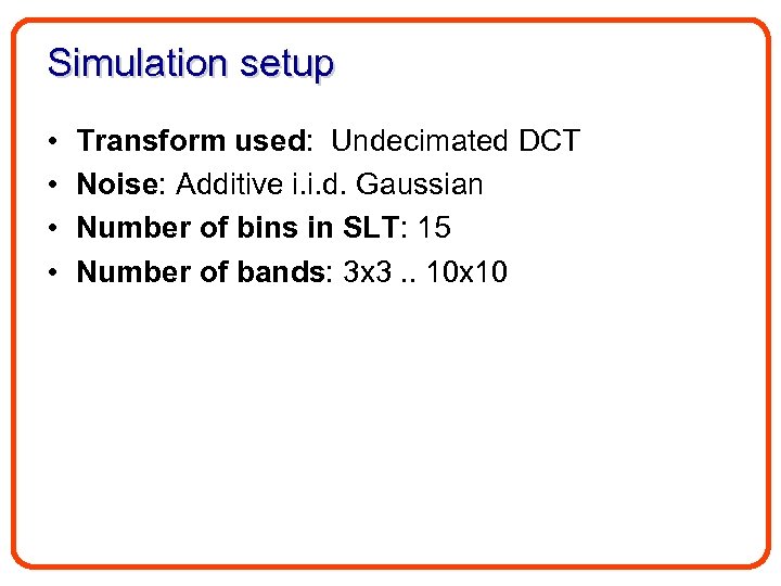Simulation setup • • Transform used: Undecimated DCT Noise: Additive i. i. d. Gaussian Number of bins in SLT: 15 Number of bands: 3 x 3. . 10 x 10

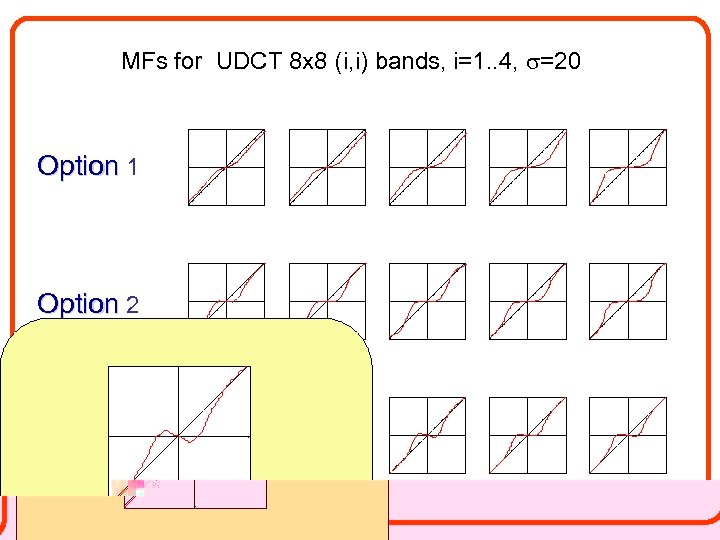MFs for UDCT 8 x 8 (i, i) bands, i=1. . 4, =20 Option 1 Option 2 Option 3

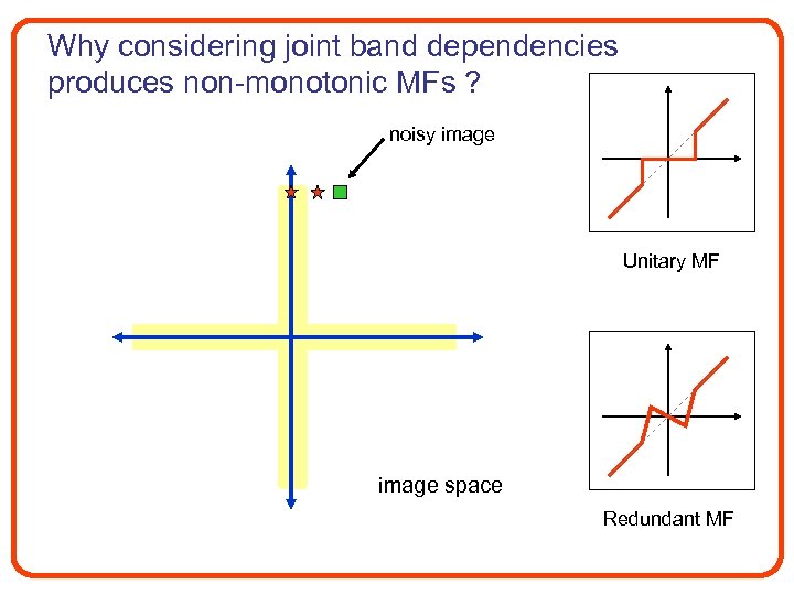Why considering joint band dependencies produces non-monotonic MFs ? noisy image Unitary MF image space Redundant MF

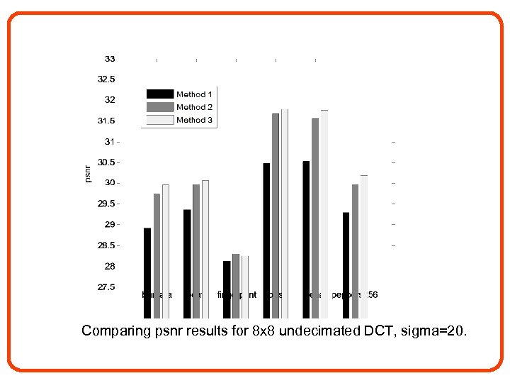Comparing psnr results for 8 x 8 undecimated DCT, sigma=20.

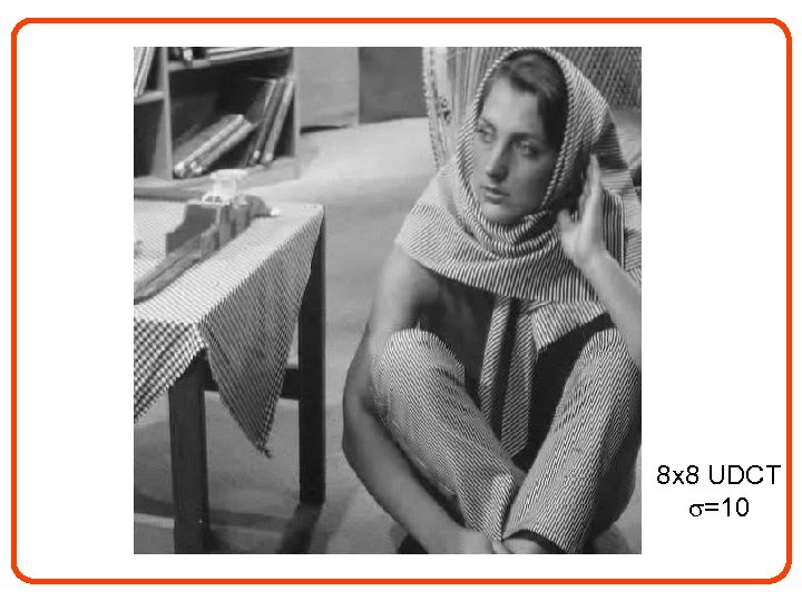8 x 8 UDCT =10

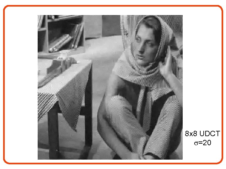8 x 8 UDCT =20

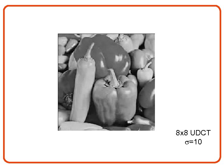8 x 8 UDCT =10

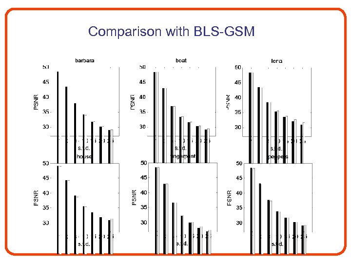Comparison with BLS-GSM

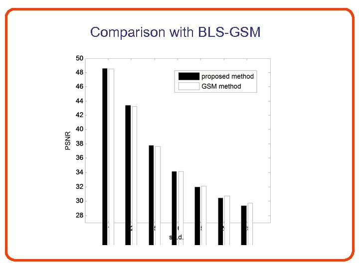Comparison with BLS-GSM

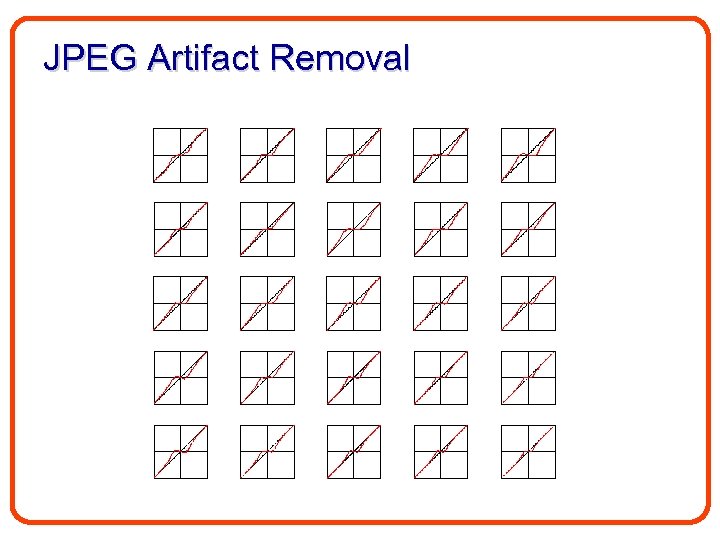
Other Degradation Models

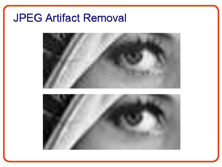JPEG Artifact Removal

JPEG Artifact Removal

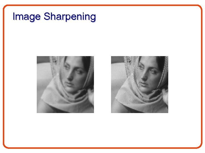Image Sharpening

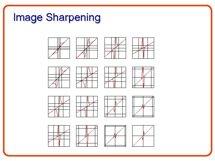Image Sharpening

Conclusions • New and simple scheme for over-complete transform based denoising. • MFs are optimized in a discriminative manner. • Linear formulation of non-linear minimization. • Eliminating the need for modeling complex statistical prior in high-dim. space. • Seamlessly applied to other degradation problems as long as scalar MFs are used for reconstruction.

Recent Results • What is the best transform to be used (for a given image or for a given set)?

Thank You