Sequence Data Mining Techniques and Applications Sunita Sarawagi

Sequence Data Mining: Techniques and Applications Sunita Sarawagi IIT Bombay Mark Craven University of Wisconsin http: //www. it. iitb. ac. in/~sunita http: //www. biostat. wisc. edu/~craven

What is a sequence? • Ordered set of elements: s = a 1, a 2, . . an • Each element ai could be – Numerical – Categorical: domain a finite set of symbols S, |S|=m – Multiple attributes • The length n of a sequence is not fixed • Order determined by time or position and could be regular or irregular

Real-life sequences • Classical applications – Speech: sequence of phonemes – Language: sequence of words and delimiters – Handwriting: sequence of strokes • Newer applications – Bioinformatics: • Genes: Sequence of 4 possible nucleotides, |S|=4 – Example: AACTGACCTGGGCCCAATCC • Proteins: Sequence of 20 possible amino-acids, |S|=20 – Example: – Telecommunications: alarms, data packets – Retail data mining: Customer behavior, sessions in a e-store (Example, Amazon) – Intrusion detection

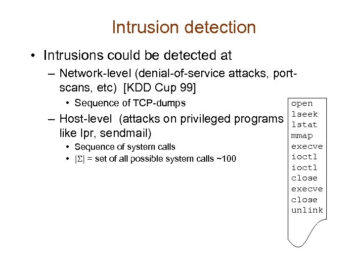Intrusion detection • Intrusions could be detected at – Network-level (denial-of-service attacks, portscans, etc) [KDD Cup 99] • Sequence of TCP-dumps – Host-level (attacks on privileged programs like lpr, sendmail) • Sequence of system calls • |S| = set of all possible system calls ~100 open lseek lstat mmap execve ioctl close execve close unlink

Outline • Traditional mining operations on sequences – Classification – Clustering – Finding repeated patterns • Primitives for handling sequence data • Sequence-specific mining operations – Partial sequence classification (Tagging) – Segmenting a sequence – Predicting next symbol of a sequence • Applications in biological sequence mining

Classification of whole sequences Given: – a set of classes C and – a number of example sequences in each class, train a model so that for an unseen sequence we can say to which class it belongs Example: – Given a set of protein families, find family of a new protein – Given a sequence of packets, label session as intrusion or normal – Given several utterances of a set of words, classify a new utterance to the right word

Conventional classification methods • Conventional classification methods assume – record data: fixed number of attributes – single record per instance to be classified (no order) • Sequences: – variable length, order important. • Adapting conventional classifiers to sequences – – Generative classifiers Boundary-based classifiers Distance based classifiers Kernel-based classifiers

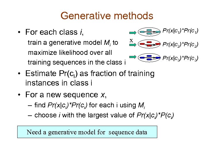Generative methods • For each class i, x train a generative model Mi to maximize likelihood over all training sequences in the class i Pr(x|c 1)*Pr(c 1) Pr(x|c 2)*Pr(c 2) Pr(x|c 3)*Pr(c 3) • Estimate Pr(ci) as fraction of training instances in class i • For a new sequence x, – find Pr(x|ci)*Pr(ci) for each i using Mi – choose i with the largest value of Pr(x|ci)*P(ci) Need a generative model for sequence data

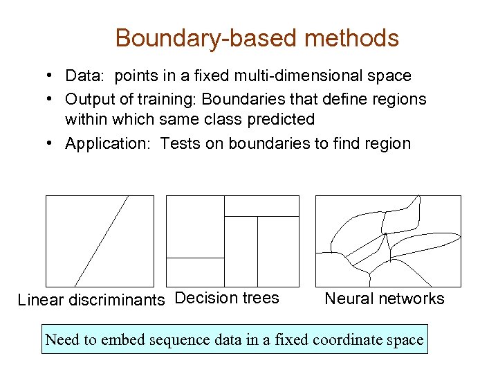Boundary-based methods • Data: points in a fixed multi-dimensional space • Output of training: Boundaries that define regions within which same class predicted • Application: Tests on boundaries to find region Linear discriminants Decision trees Neural networks Need to embed sequence data in a fixed coordinate space

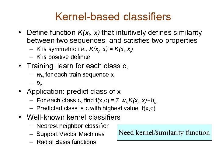Kernel-based classifiers • Define function K(xi, x) that intuitively defines similarity between two sequences and satisfies two properties – K is symmetric i. e. , K(xi, x) = K(x, xi) – K is positive definite • Training: learn for each class c, – wic for each train sequence xi – bc • Application: predict class of x – For each class c, find f(x, c) = S wic. K(xi, x)+bc – Predicted class is c with highest value f(x, c) • Well-known kernel classifiers – Nearest neighbor classifier – Support Vector Machines – Radial Basis functions Need kernel/similarity function

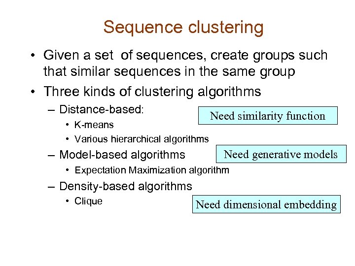Sequence clustering • Given a set of sequences, create groups such that similar sequences in the same group • Three kinds of clustering algorithms – Distance-based: • K-means • Various hierarchical algorithms – Model-based algorithms Need similarity function Need generative models • Expectation Maximization algorithm – Density-based algorithms • Clique Need dimensional embedding

Outline • Traditional mining on sequences • Primitives for handling sequence data – Embed sequence in a fixed dimensional space • All conventional record mining techniques will apply – Generative models for sequence • Sequence classification: generative methods • Clustering sequences: model-based approach – Distance between two sequences • Sequence classification: SVM and NN • Clustering sequences: distance-based approach • Sequence-specific mining operations • Applications

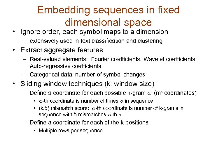Embedding sequences in fixed dimensional space • Ignore order, each symbol maps to a dimension – extensively used in text classification and clustering • Extract aggregate features – Real-valued elements: Fourier coefficients, Wavelet coefficients, Auto-regressive coefficients – Categorical data: number of symbol changes • Sliding window techniques (k: window size) – Define a coordinate for each possible k-gram a (mk coordinates) • a-th coordinate is number of times a in sequence • (k, b) mismatch score: a-th coordinate is number of k-grams in sequence with b mismatches with a – Define a coordinate for each of the k-positions • Multiple rows per sequence

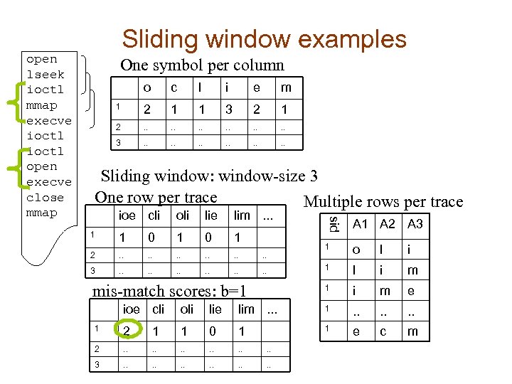One symbol per column o c l i e m 1 2 1 1 3 2 1 2 . . . 3 . . . Sliding window: window-size 3 One row per trace Multiple rows per trace ioe cli oli lie lim. . . 1 1 0 1 2 . . . 3 . . . A 1 A 2 A 3 1 o l i 1 l i m 1 mis-match scores: b=1 sid open lseek ioctl mmap execve ioctl open execve close mmap Sliding window examples i m e ioe cli oli lie lim. . . 1 2 1 1 0 1 1 e c m 2 . . . 3 . . .

Detecting attacks on privileged programs • • Short sequences of system calls made during normal execution of system calls are very consistent, yet different from the sequences of its abnormal executions Two approaches – STIDE (Warrender 1999) • Create dictionary of unique k-windows in normal traces, count what fraction occur in new traces and threshold. – RIPPER –based (Lee 1998) • next. . .

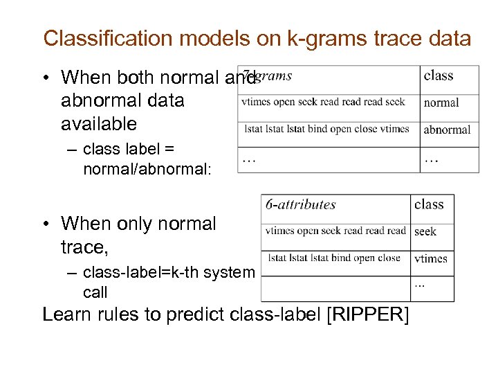Classification models on k-grams trace data • When both normal and abnormal data available – class label = normal/abnormal: • When only normal trace, – class-label=k-th system call Learn rules to predict class-label [RIPPER]

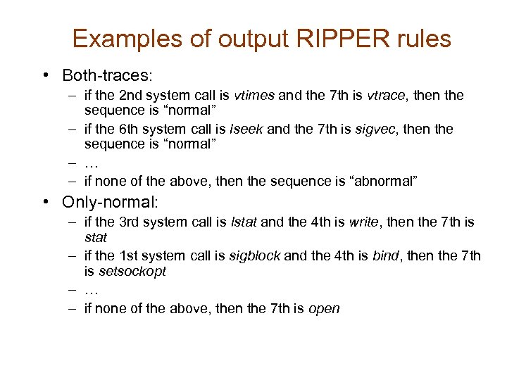Examples of output RIPPER rules • Both-traces: – if the 2 nd system call is vtimes and the 7 th is vtrace, then the sequence is “normal” – if the 6 th system call is lseek and the 7 th is sigvec, then the sequence is “normal” – … – if none of the above, then the sequence is “abnormal” • Only-normal: – if the 3 rd system call is lstat and the 4 th is write, then the 7 th is stat – if the 1 st system call is sigblock and the 4 th is bind, then the 7 th is setsockopt – … – if none of the above, then the 7 th is open

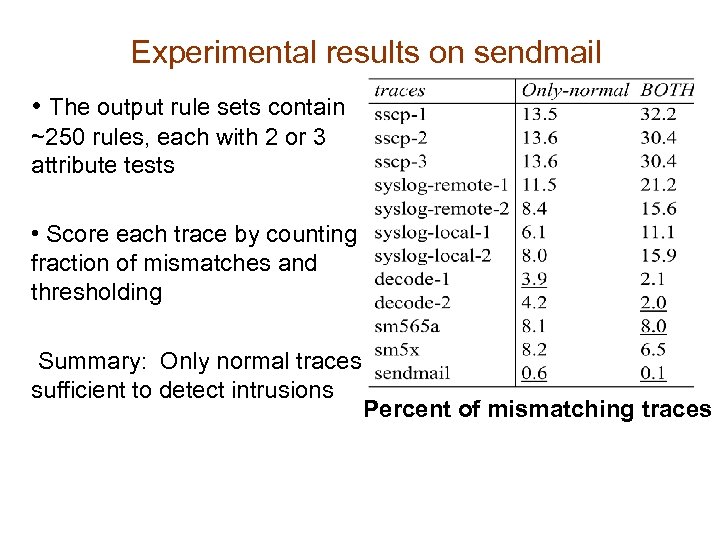Experimental results on sendmail • The output rule sets contain ~250 rules, each with 2 or 3 attribute tests • Score each trace by counting fraction of mismatches and thresholding Summary: Only normal traces sufficient to detect intrusions Percent of mismatching traces

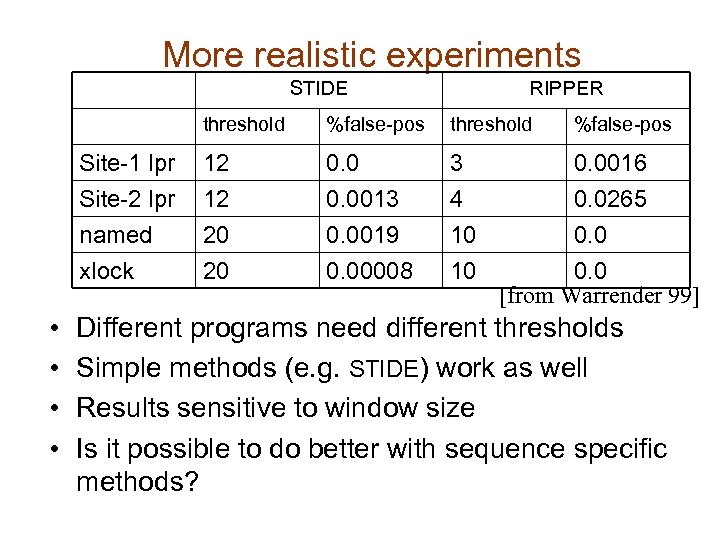More realistic experiments STIDE RIPPER threshold %false-pos Site-1 lpr Site-2 lpr 12 12 0. 0013 3 4 0. 0016 0. 0265 named xlock • • %false-pos 20 20 0. 0019 0. 00008 10 10 0. 0 [from Warrender 99] Different programs need different thresholds Simple methods (e. g. STIDE) work as well Results sensitive to window size Is it possible to do better with sequence specific methods?

Outline • Traditional mining on sequences • Primitives for handling sequence data – Embed sequence in a fixed dimensional space • All conventional record mining techniques will apply – Distance between two sequences • Sequence classification: SVM and NN • Clustering sequences: distance-based approach – Generative models for sequences • Sequence classification: whole and partial • Clustering sequences: model-based approach • Sequence-specific mining operations • Applications in biological sequence mining

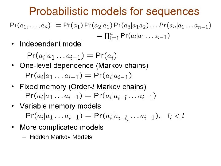Probabilistic models for sequences • Independent model • One-level dependence (Markov chains) • Fixed memory (Order-l Markov chains) • Variable memory models • More complicated models – Hidden Markov Models

Independent model • Model structure – A parameter for each symbol in S • Probability of a sequence s being generated from the model – example: Pr(AACA) = Pr(A) Pr(C) Pr(A) = Pr(A)3 Pr(C) = 0. 13 ´ 0. 9 • Training transition probabilities – Data T : set of sequences – Count(s ε T): total number of times substring s appears in training data T Pr(s) = Count(s ε T) / length(T) Pr(A) = 0. 1 Pr(C) = 0. 9

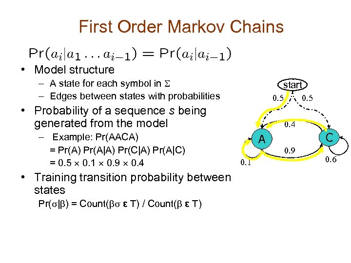First Order Markov Chains • Model structure – A state for each symbol in S – Edges between states with probabilities start 0. 5 • Probability of a sequence s being generated from the model – Example: Pr(AACA) = Pr(A) Pr(A|A) Pr(C|A) Pr(A|C) = 0. 5 ´ 0. 1 ´ 0. 9 ´ 0. 4 • Training transition probability between states Pr(s|b) = Count(bs ε T) / Count(b ε T) 0. 5 0. 4 A 0. 1 C 0. 9 0. 6

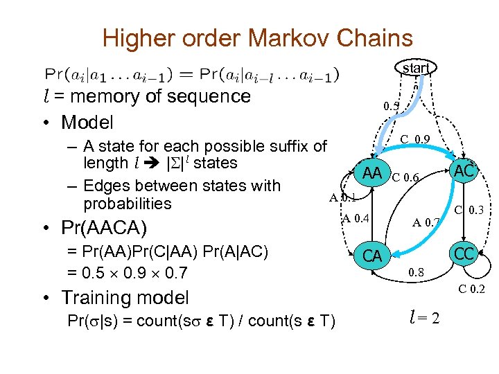Higher order Markov Chains start l = memory of sequence • Model 0. 5 – A state for each possible suffix of length l |S|l states AA – Edges between states with A 0. 1 probabilities • Pr(AACA) = Pr(AA)Pr(C|AA) Pr(A|AC) = 0. 5 ´ 0. 9 ´ 0. 7 • Training model Pr(s|s) = count(ss ε T) / count(s ε T) A 0. 4 CA C 0. 9 C 0. 6 A 0. 7 AC C 0. 3 CC 0. 8 C 0. 2 l = 2

Variable Memory models start • Probabilistic Suffix Automata (PSA) • Model – States: substrings of size no greater than l where no string is suffix of another • Calculating Pr(AACA): = Pr(A)Pr(A|A)Pr(C|A)Pr(A|AC) = 0. 5 ´ 0. 3 ´ 0. 7 ´ 0. 1 0. 2 0. 5 C 0. 9 CC AC C 0. 7 A 0. 1 • Training: not straight-forward – Eased by Prediction Suffix Trees – PSTs can be converted to PSA after training C 0. 6 A A 0. 3 A 0. 6

Prediction Suffix Trees (PSTs) • Suffix trees with emission probabilities of observation attached with each tree node C 0. 9 CC AC C 0. 7 A 0. 1 C 0. 6 A A 0. 3 0. 28, 0. 72 0. 3, 0. 7 A e C 0. 25, 0. 75 AC CC 0. 4, 0. 6 Pr(AACA)=0. 28 ´ 0. 3 ´ 0. 7 ´ 0. 1, 0. 9 • Linear time algorithms exist for constructing such PSTs from training data [Apostolico 2000]

Hidden Markov Models • Doubly stochastic models A 0. 6 A 0. 9 C 0. 5 0. 1 S 1 – Finding Pr(S) – The highest probability path P that maximizes Pr(S|P) (Viterbi) • Training the model – (Baum-Welch algorithm) 0. 4 S 2 0. 5 0. 1 • Efficient dynamic programming algorithms exist for 0. 9 C 0. 8 S 3 S 4 A 0. 5 0. 2 A 0. 3 C C 0. 5 0. 7

Discriminative training of HMMs • Models trained to maximize likelihood of data might perform badly when – Model not representative of data – Training data insufficient • Alternatives to Maximum-likelihood/EM – Objective functions: • Minimum classification error • Maximum posterior probability of actual label Pr(c|x) • Maximum mutual information with class – Harder to train above functions, number of alternatives to EM proposed • Generalized probabilistic descent [Katagiri 98] • Deterministic annealing [Rao 01]

HMMs for profiling system calls • Training: – Initial number of states = 40 (roughly equals number of distinct system calls) – Train on normal traces • Testing: – Need to handle variable length and online data – For each call, find the total probability of outputting given all calls before it. • If probability below a threshold call it abnormal. – Trace is abnormal if fraction of abnormal calls are high

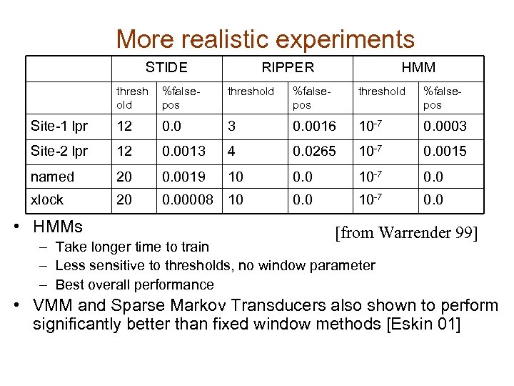More realistic experiments STIDE RIPPER HMM thresh old %falsepos threshold %falsepos Site-1 lpr 12 0. 0 3 0. 0016 10 -7 0. 0003 Site-2 lpr 12 0. 0013 4 0. 0265 10 -7 0. 0015 named 20 0. 0019 10 0. 0 10 -7 0. 0 xlock 20 0. 00008 10 0. 0 10 -7 0. 0 • HMMs [from Warrender 99] – Take longer time to train – Less sensitive to thresholds, no window parameter – Best overall performance • VMM and Sparse Markov Transducers also shown to perform significantly better than fixed window methods [Eskin 01]

ROC curves comparing different methods [from Warrender 99]

Outline • Traditional mining on sequences • Primitives for handling sequence data • Sequence-specific mining operations – Partial sequence classification (Tagging) – Segmenting a sequence – Predicting next symbol of a sequence • Applications in biological sequence mining

Partial sequence classification (Tagging) • The tagging problem: – Given: • A set of tags L • Training examples of sequences showing the breakup of the sequence into the set of tags – Learn to breakup a sequence into tags – (classification of parts of sequences) • Examples: – Text segmentation • Break sequence of words forming an address string into subparts like Road, City name etc – Continuous speech recognition • Identify words in continuous speech

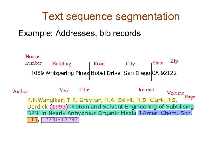Text sequence segmentation Example: Addresses, bib records House number Building Road City State Zip 4089 Whispering Pines Nobel Drive San Diego CA 92122 Author Year Title Journal Volume Page P. P. Wangikar, T. P. Graycar, D. A. Estell, D. S. Clark, J. S. Dordick (1993) Protein and Solvent Engineering of Subtilising BPN' in Nearly Anhydrous Organic Media J. Amer. Chem. Soc. 115, 12231 -12237.

Approaches used for tagging • Learn to identify start and end boundaries of each label – Method: for each label, build two classifiers for accepting its two boundaries. – Any conventional classifier would do: • Rule-based most common. • K-windows approach: – For each label, train a classifier on k-windows – During testing • classify each k-window • Adapt state-based generative models like HMM

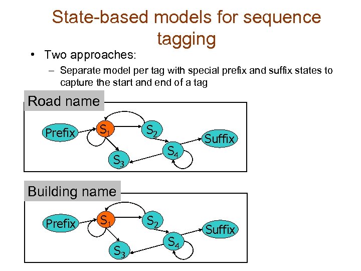State-based models for sequence tagging • Two approaches: – Separate model per tag with special prefix and suffix states to capture the start and end of a tag Road name Prefix S 1 S 2 S 4 S 3 Suffix Building name Prefix S 1 S 2 S 3 S 4 Suffix

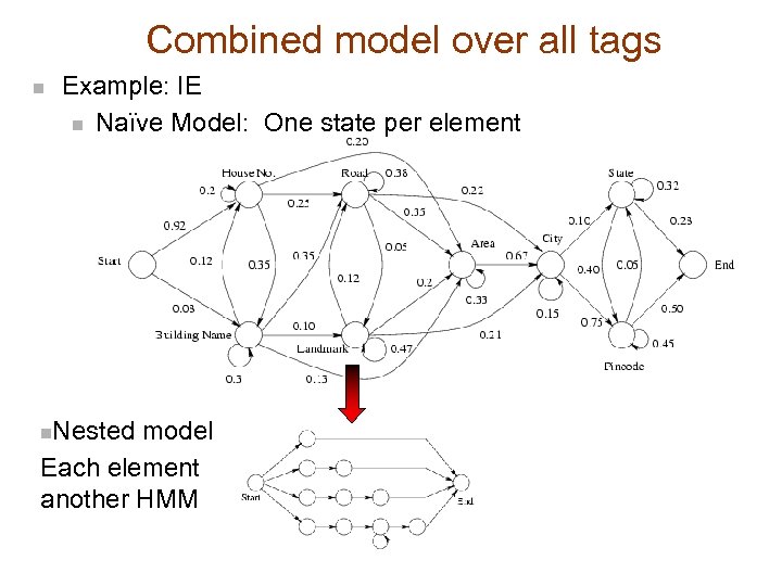Combined model over all tags n Example: IE n Naïve Model: One state per element … Mahatma Gandhi Road Near Parkland. . . Nested model Each element another HMM … [Mahatma Gandhi Road Near : Landmark] Parkland. . . n

Other approaches • Disadvantages of generative models (HMMs) – Maximizing joint probability of sequence and labels may not maximize accuracy – Conditional independence of features a restrictive assumption • Alternative: Conditional Random Fields – Maximize conditional probability of labels given sequence – Arbitrary overlapping features allowed

Outline • Traditional mining on sequences • Primitives for handling sequence data • Sequence-specific mining operations – Partial sequence classification (Tagging) – Segmenting a sequence – Predicting next symbol of a sequence • Applications in biological sequence mining

Segmenting sequences Basic premise: Sequence assumed to be generated from multiple models Goal: discover boundaries of model change Applications: Bioinformatics Better models by breaking up heterogeneous sequences Return A Pick B

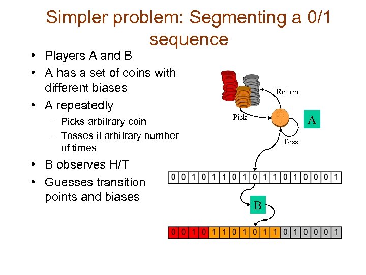Simpler problem: Segmenting a 0/1 sequence • Players A and B • A has a set of coins with different biases • A repeatedly – Picks arbitrary coin – Tosses it arbitrary number of times • B observes H/T • Guesses transition points and biases Return Pick A Toss B

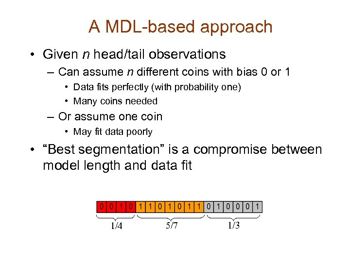A MDL-based approach • Given n head/tail observations – Can assume n different coins with bias 0 or 1 • Data fits perfectly (with probability one) • Many coins needed – Or assume one coin • May fit data poorly • “Best segmentation” is a compromise between model length and data fit 1/4 5/7 1/3

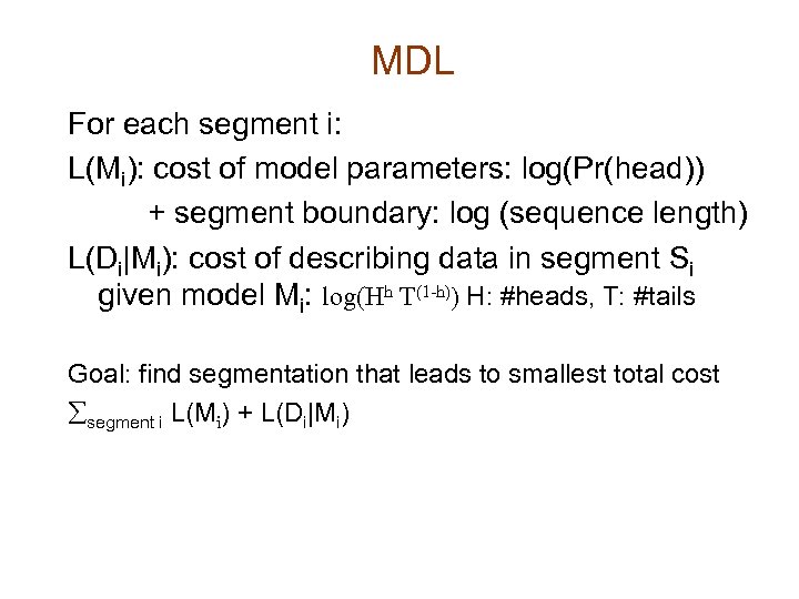MDL For each segment i: L(Mi): cost of model parameters: log(Pr(head)) + segment boundary: log (sequence length) L(Di|Mi): cost of describing data in segment Si given model Mi: log(Hh T(1 -h)) H: #heads, T: #tails Goal: find segmentation that leads to smallest total cost åsegment i L(Mi) + L(Di|Mi)

How to find optimal segments Sequence of 17 tosses: Derived graph with 18 nodes and all possible edges Shortest path Edge cost = model cost + data cost

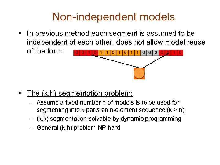Non-independent models • In previous method each segment is assumed to be independent of each other, does not allow model reuse of the form: • The (k, h) segmentation problem: – Assume a fixed number h of models is to be used for segmenting into k parts an n-element sequence (k > h) – (k, k) segmentation solvable by dynamic programming – General (k, h) problem NP hard

Approximations: for (k, h) segmentation 1. Solve (k, k) to get segments S 1 S 2 S 3 S 4 2. Solve (n, h) to get H models – Example: 2 -medians M 1 M 2 3. Assign each segment to best of H A second variant (Replace step 2 above with) – Find summary statistics for each k segment, cluster them into H clusters

Results of segmenting genetic sequences From: Gionis & Mannila 2003

Outline • • • Traditional mining operations on sequences Primitives for handling sequence data Sequence-specific mining operations • Applications in biological sequence mining 1. Classifying proteins according to family 2. Finding genes in DNA sequences

Two sequence mining applications

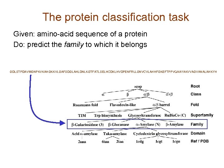The protein classification task Given: amino-acid sequence of a protein Do: predict the family to which it belongs GDLSTPDAVMGNPKVKAHGKKVLGAFSDGLAHLDNLKGTFATLSELHCDKLHVDPENFRLLGNVCVLAHHFGKEFTPPVQAAYAKVVAGVANALAHKYH

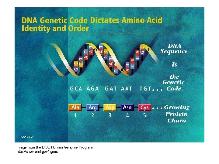image from the DOE Human Genome Program http: //www. ornl. gov/hgmis

The roles of proteins • A protein family is… Figure from the DOE Human Genome Program http: //www. ornl. gov/hgmis

The roles of proteins • The amino-acid sequence of a protein determines its structure • The structure of a protein determines its function • Proteins play many key roles in cells – structural support – storage of amino acids – transport of other substances – coordination of an organism’s activities – response of cell to chemical stimuli – movement – protection against disease – selective acceleration of chemical reactions

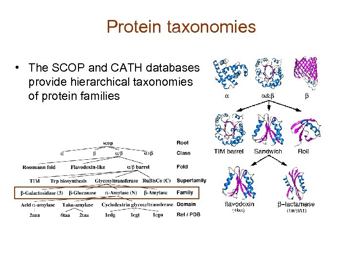Protein taxonomies • The SCOP and CATH databases provide hierarchical taxonomies of protein families

An alignment of globin family proteins n n The sequences in a family may vary in length Some positions are more conserved than others Figure from www-cryst. bioc. cam. ac. uk/~max/res_globin. html

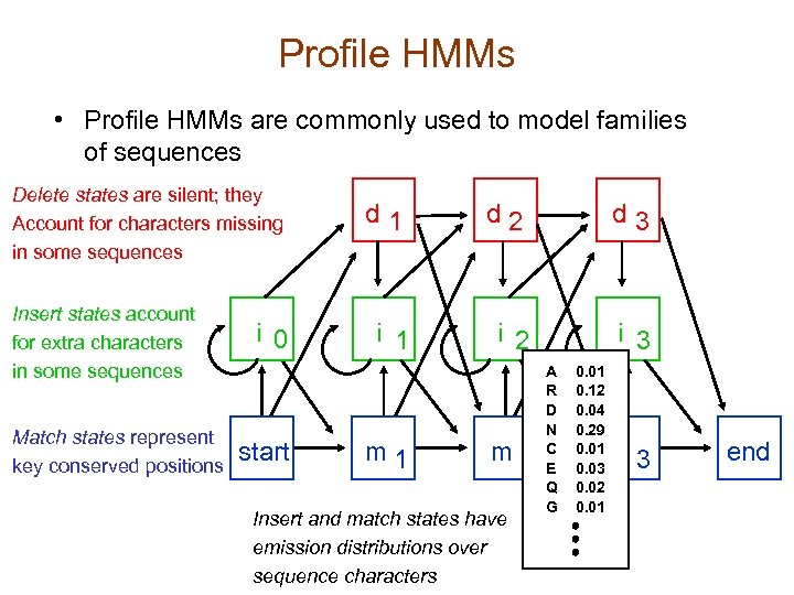Profile HMMs • Profile HMMs are commonly used to model families of sequences Delete states are silent; they Account for characters missing in some sequences Insert states account for extra characters in some sequences Match states represent key conserved positions i 0 start d 1 d 2 d 3 i 1 i 2 i 3 m 1 m 2 Insert and match states have emission distributions over sequence characters A R D N C E Q G 0. 01 0. 12 0. 04 0. 29 0. 01 0. 03 0. 02 0. 01 m 3 end

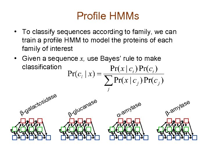Profile HMMs • To classify sequences according to family, we can train a profile HMM to model the proteins of each family of interest • Given a sequence x, use Bayes’ rule to make classification se la -ga β a sid cto l β -g ase can u α-a e las my β-a m e las y

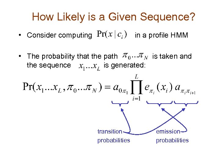How Likely is a Given Sequence? • Consider computing in a profile HMM • The probability that the path is taken and the sequence is generated: transition probabilities emission probabilities

How Likely Is A Given Sequence? 0. 4 0. 2 0. 5 A C G T 0. 4 0. 1 0. 2 0. 3 0. 8 A C G T 1 begin 0 0. 5 A C G T 0. 4 0. 1 0. 4 0. 6 3 0. 2 2 0. 8 0. 2 0. 3 0. 2 A C G T 0. 1 0. 4 0. 1 end 5 0. 9

How Likely is a Given Sequence? • the probability over all paths is: • but the number of paths can be exponential in the length of the sequence. . . • the Forward algorithm enables us to compute this efficiently using dynamic programming

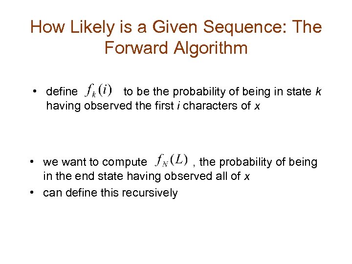How Likely is a Given Sequence: The Forward Algorithm • define to be the probability of being in state k having observed the first i characters of x • we want to compute , the probability of being in the end state having observed all of x • can define this recursively

The Forward Algorithm • initialization: probability that we’re in start state and have observed 0 characters from the sequence • recursion for emitting states (i =1…L): • recursion for silent states: • termination: probability that we’re in the end state and have observed the entire sequence

Training a profile HMM • The parameters in profile HMMs are typically trained using the Baum-Welch method (an EM algorithm) • Heuristic methods are used to determine the length of the model – Initialize using an alignment of the training sequences (as in globin example) – Iteratively make local adjustments to length if delete or insert states are used “too much” for training sequences

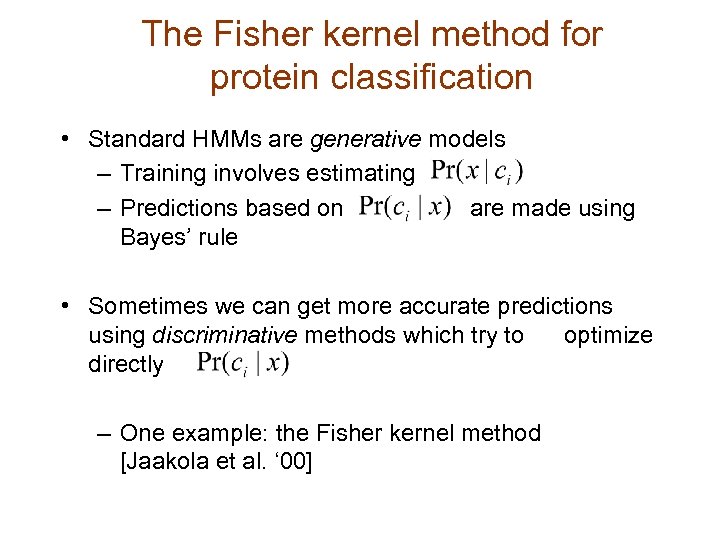The Fisher kernel method for protein classification • Standard HMMs are generative models – Training involves estimating – Predictions based on are made using Bayes’ rule • Sometimes we can get more accurate predictions using discriminative methods which try to optimize directly – One example: the Fisher kernel method [Jaakola et al. ‘ 00]

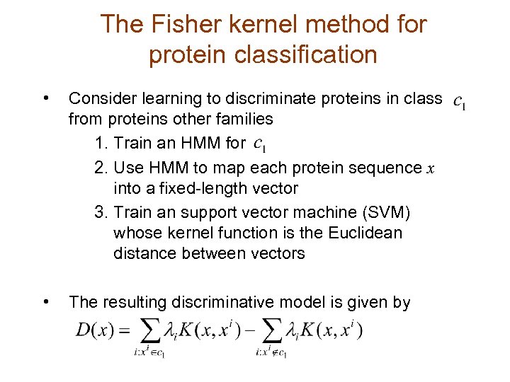The Fisher kernel method for protein classification • Consider learning to discriminate proteins in class from proteins other families 1. Train an HMM for 2. Use HMM to map each protein sequence x into a fixed-length vector 3. Train an support vector machine (SVM) whose kernel function is the Euclidean distance between vectors • The resulting discriminative model is given by

The Fisher kernel method for protein classification • How can we get an informative fixed-length vector? Compute the Fisher score i. e. each component of is a derivative of the log-likelihood of x with respect to a particular parameter in the HMM

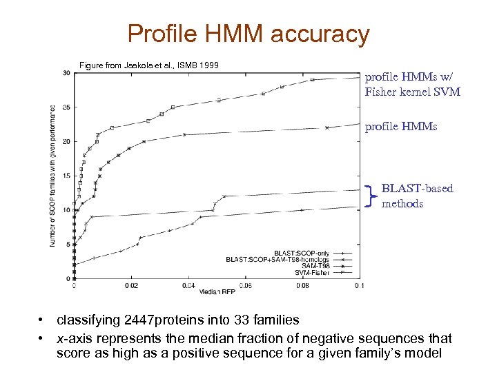Profile HMM accuracy Figure from Jaakola et al. , ISMB 1999 profile HMMs w/ Fisher kernel SVM profile HMMs BLAST-based methods • classifying 2447 proteins into 33 families • x-axis represents the median fraction of negative sequences that score as high as a positive sequence for a given family’s model

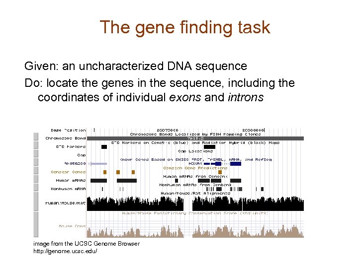The gene finding task Given: an uncharacterized DNA sequence Do: locate the genes in the sequence, including the coordinates of individual exons and introns image from the UCSC Genome Browser http: //genome. ucsc. edu/

image from the DOE Human Genome Program http: //www. ornl. gov/hgmis

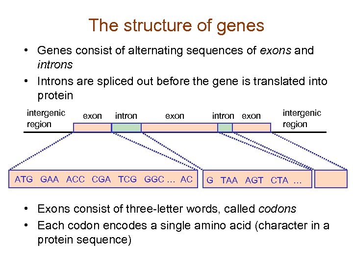The structure of genes • Genes consist of alternating sequences of exons and introns • Introns are spliced out before the gene is translated into protein intergenic region exon intron exon ATG GAA ACC CGA TCG GGC … AC intron exon intergenic region G TAA AGT CTA … • Exons consist of three-letter words, called codons • Each codon encodes a single amino acid (character in a protein sequence)

The GENSCAN HMM for gene finding [Burge & Karlin ‘ 97] Each shape represents a functional unit of a gene or genomic region Pairs of intron/exon units represent the different ways an intron can interrupt a coding sequence (after 1 st base in codon, after 2 nd base or after 3 rd base) Complementary submodel (not shown) detects genes on opposite DNA strand

The GENSCAN HMM • For each sequence type, GENSCAN models – the length distribution – the sequence composition • Length distribution models vary depending on sequence type – Nonparametric (using histograms) – Parametric (using geometric distributions) – Fixed-length • Sequence composition models vary depending on type – 5 th-order, inhomogeneous – 5 th -order homogenous – Independent and 1 st-order inhomogeneous – Tree-structured variable memory

Representing exons in GENSCAN • For exons, GENSCAN uses – Histograms to represent exon lengths – 5 th-order, inhomogeneous Markov models to represent exon sequences • 5 th-order, inhomogeneous models can represent statistics about pairs of neighboring codons

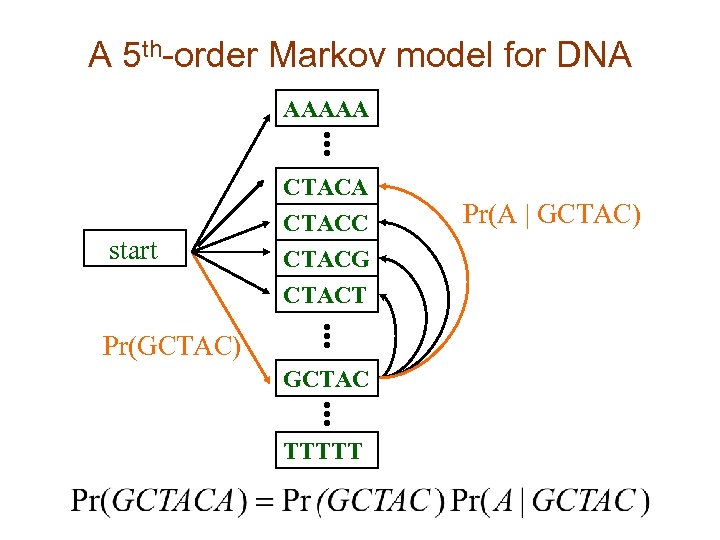A 5 th-order Markov model for DNA AAAAA start CTACA CTACC CTACG CTACT Pr(GCTAC) GCTAC TTTTT Pr(A | GCTAC)

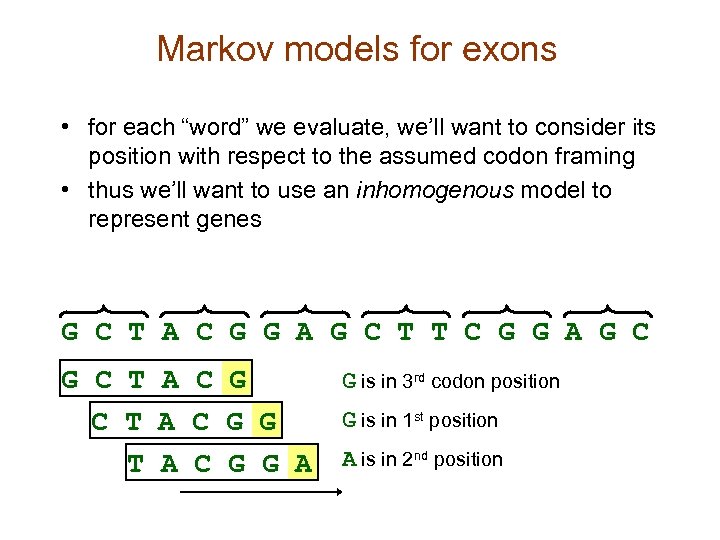Markov models for exons • for each “word” we evaluate, we’ll want to consider its position with respect to the assumed codon framing • thus we’ll want to use an inhomogenous model to represent genes G C T A C G G A G C T T C G G A G C T A C G G A G is in 3 rd codon position G is in 1 st position A is in 2 nd position

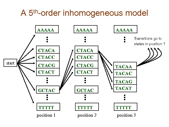A 5 th-order inhomogeneous model AAAAA Transitions go to states in position 1 CTACA CTACC start CTACA CTACC CTACG CTACT TACAA TACAC GCTAC TACAG TACAT TTTTT position 2 position 3 position 1

Inference with the gene-finding HMM given: an uncharacterized DNA sequence do: find the most probable path through the model for the sequence • This path will specify the coordinates of the predicted genes (including intron and exon boundaries) • The Viterbi algorithm is used to compute this path

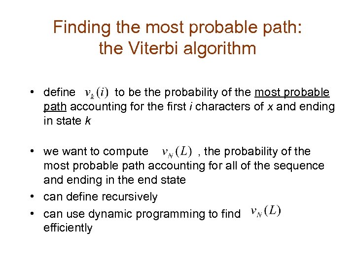Finding the most probable path: the Viterbi algorithm • define to be the probability of the most probable path accounting for the first i characters of x and ending in state k • we want to compute , the probability of the most probable path accounting for all of the sequence and ending in the end state • can define recursively • can use dynamic programming to find efficiently

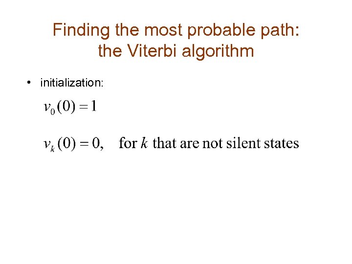Finding the most probable path: the Viterbi algorithm • initialization:

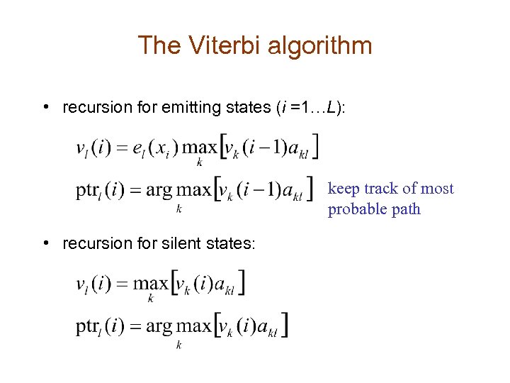The Viterbi algorithm • recursion for emitting states (i =1…L): keep track of most probable path • recursion for silent states:

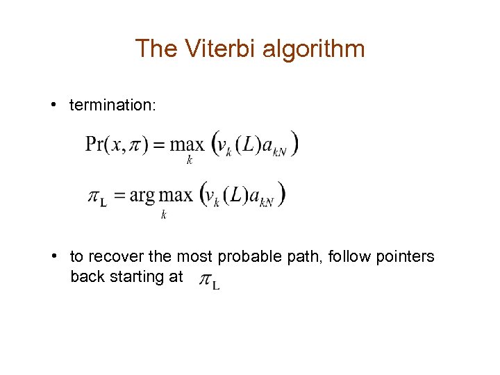The Viterbi algorithm • termination: • to recover the most probable path, follow pointers back starting at

Parsing a DNA Sequence The Viterbi path represents a parse of a given sequence, predicting exons, introns, etc ACCGTTACGTGTCATTCTACGTGATCATCGGATCCTAGAATCATCGATCCGTGCGATCGGATTAGCTTAGCTAGGAGAGCATCGGATCGAGGAGGAGCCTATATAAATCAA

Some lessons from these biological applications • HMMs provide state-of-the-art performance in protein classification and gene finding • HMMs can naturally classify and parse sequences of variable length • Much domain knowledge can be incorporated into the structure of the models – Types, lengths and ordering of sequence features – Appropriate amount of memory to represent various sequence features • Models can vary representation across sequence features • Discriminative methods often provide superior predictive accuracy to generative methods

• • • References S. F. Altschul, T. L. Madden, A. A. Schaffer, J. Zhang, Z. Zhang, W. Miller, and D. J. Lipman. Gapped BLAST and PSI-BLAST: A new generation of protein database search programs. Nucleic Acids Research, 25: 3389– 3402, 1997. Apostolico, A. , and Bejerano, G. 2000. Optimal amnesic probabilistic automata or how to learn and classify proteins in linear time and space. In Proceedings of RECOMB 2000. http: //citeseer. nj. nec. com/apostolico 00 optimal. html Vinayak R. Borkar, Kaustubh Deshmukh, and Sunita Sarawagi. Automatic text segmentation for extracting structured records. SIGMOD 2001. C. Burge and S. Karlin, Prediction of Complete Gene Structures in Human Genomic DNA. Journal of Molecular Biology, 268: 78 -94, 1997. Mary Elaine Calif and R. J. Mooney. Relational learning of pattern-match rules for information extraction. AAAI 1999. S. Chakrabarti, S. Sarawagi and B. Dom, Mining surprising patterns using temporal description length, VLDB, 1998 M. Collins, “Discriminitive training method for Hidden Markov Models: Theory and experiments with perceptron algorithms, EMNLP 2002 R. Durbin, S. Eddy, A. Krogh, and G. Mitchison, Biological sequence analysis: probabilistic models of proteins and nucleic acids, Cambridge University Press, 1998. Eleazar Eskin, Wenke Lee and Salvatore J. Stolfo. ``Modeling System Calls for Intrusion Detection with Dynamic Window Sizes. '' Proceedings of DISCEX II. June 2001. IDS http: //www. cs. columbia. edu/ids/publications/ D Freitag and A Mc. Callum, Information Extraction with HMM Structures Learned by Stochastic Optimization, AAAI 2000

• • • References Gionis and H. Mannila: Finding recurrent sources in sequences. ACM Re. COMB 2003 Michael T. Goodrich, Efficient Piecewise-Approximation Using the Uniform Metric Symposium on Computational Geometry , (1994) D. Haussler. Convolution kernels on discrete structure. Technical report, UC Santa Cruz, 1999. K. Karplus, C. Barrett, and R. Hughey, Hidden Markov models for detecting remote protein homologies. Bioinformatics 14(10): 846 -856, 1998. L. Lo Conte, S. Brenner, T. Hubbard, C. Chothia, and A. Murzin. SCOP database in 2002: refinements accommodate structural genomics. Nucleic Acids Research, 30: 264267, 2002 Wenke Lee and Sal Stolfo. ``Data Mining Approaches for Intrusion Detection'' In Proceedings of the Seventh USENIX Security Symposium (SECURITY '98), San Antonio, TX, January 1998 A. Mc. Callum and D. Freitag and F. Pereira, Maximum entropy Markov models for information extraction and segmentation, ICML-2000 Rabiner, Lawrence R. , 1990. A tutorial on hidden Markov models and selected applications in speech recognition. In Alex Weibel and Kay-Fu Lee (eds. ), Readings in Speech Recognition. Los Altos, CA: Morgan Kaufmann, pages 267 --296. D. Ron, Y. Singer and N. Tishby. The power of amnesia: learning probabilistic automata with variable memory length. Machine Learning, 25: 117 -- 149, 1996 Warrender, Christina, Stephanie Forrest, and Barak Pearlmutter. Detecting Intrusions Using System Calls: Alternative Data Models. To appear, 1999 IEEE Symposium on Security and Privacy. 1999