Seminar in Auctions and Mechanism Design Chapter 4

Seminar in Auctions and Mechanism Design Chapter 4 Bayesian Approximation By: Yotam Eliraz 037026382 & Gilad Shohat Based on Chapter 4 on Jason Hartline’s book

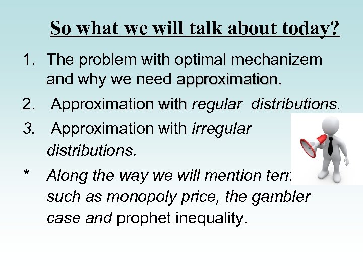So what we will talk about today? 1. The problem with optimal mechanizem and why we need approximation. 2. Approximation with regular distributions. 3. Approximation with irregular distributions. * Along the way we will mention terms such as monopoly price, the gambler case and prophet inequality.

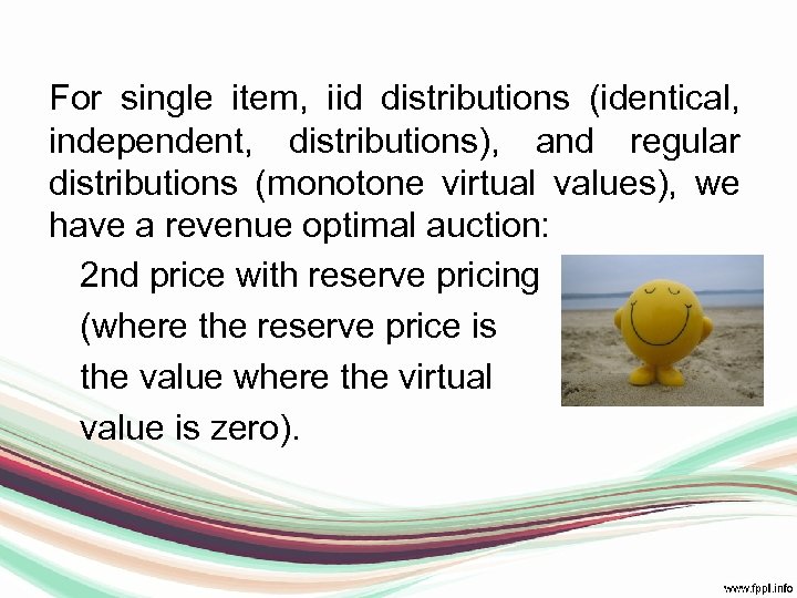For single item, iid distributions (identical, independent, distributions), and regular distributions (monotone virtual values), we have a revenue optimal auction: 2 nd price with reserve pricing (where the reserve price is the value where the virtual value is zero).

Chapter 3 also shows For any regular distribution, Maximizing social welfare with virtual values has the effect of maximizing profit The expected profit is equal to the expected virtual social welfare However: Maximizing social welfare need not be simple to do or describe. And, does not translate to reserves

Approximation (1) • Single reserve price mechanisms only work well (maximize profit) if iid, regular, single item • We would like to show that although reserve-price-based mechanisms are not always optimal, they can be approximately optimal in a wide range of environments.

Approximation (2) • The approximation factor is the ratio between the optimal soultion and the one we obtain

Non identical distributions, single item, Mechanism 4. 1: For a second-price auction with reserves r = (r 1 , . . . , rn ) the algorithm is as following: 1. reject each agent i with vi

Consider 3 bidders with Distributions F 1= U[0, 1], F 2 = U[0, 2] and F 3 =U[0, 3], respectively F 1(v) = v, f 1(v) = 1, F 2(v) = v/2, f 2(v)=1/2 F 3(v) = v/3, f 3(v)=1/3 The virtual value of all agents with distribution density f and cumulative distribution F is v – (1 - F(v))/f(v) The reserve for agent 1 is r 1 such that r 1 – (1 - F 1(r 1))/f 1(r 1) = 0 Or r 1 – (1 – r 1)/1 = 0, or 2 r 1 = 1, or r 1 = ½ The reserve for agent 2 is r 2 such that r 2 – (1 - F 2(r 2))/f 2(r 2) = 0 Or r 2 – (1 – r 2/2)*2 = 0, or 2 = 2, or r 2=1, r 3 = 1. 5,

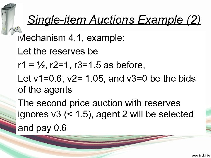Single-item Auctions Example (2) Mechanism 4. 1, example: Let the reserves be r 1 = ½, r 2=1, r 3=1. 5 as before, Let v 1=0. 6, v 2= 1. 05, and v 3=0 be the bids of the agents The second price auction with reserves ignores v 3 (< 1. 5), agent 2 will be selected and pay 0. 6

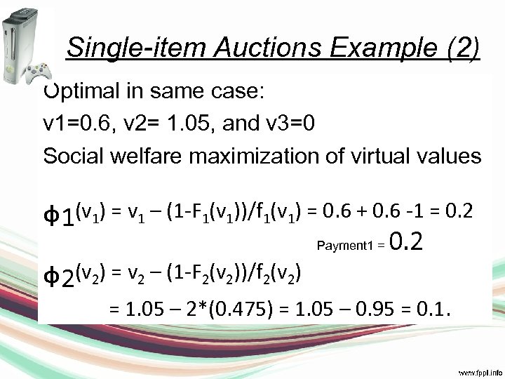Single-item Auctions Example (2) Optimal in same case: v 1=0. 6, v 2= 1. 05, and v 3=0 Social welfare maximization of virtual values ᵩ 1(v ) = v – (1 -F (v ))/f (v ) = 0. 6 + 0. 6 -1 = 0. 2 ᵩ 2(v ) = v – (1 -F (v ))/f (v ) 1 1 1 Payment 1 = 2 2 2 = 1. 05 – 2*(0. 475) = 1. 05 – 0. 95 = 0. 1.

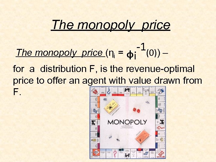The monopoly price -1(0)) – The monopoly price (ηi = ᵩi for a distribution F, is the revenue-optimal price to offer an agent with value drawn from F.

Fact Any agent whose value exceeds the monopoly price has non-negative virtual value. (For regular distributions – monotone virtual prices).

The approximation part The expected revenue of the second-price auction with monopoly reserves is close to the optimal revenue when the distributions are regular. Why close? Why not the same? ? ? Did we not prove that this is optimal? ? ? NO!! NOT IID, not identical.

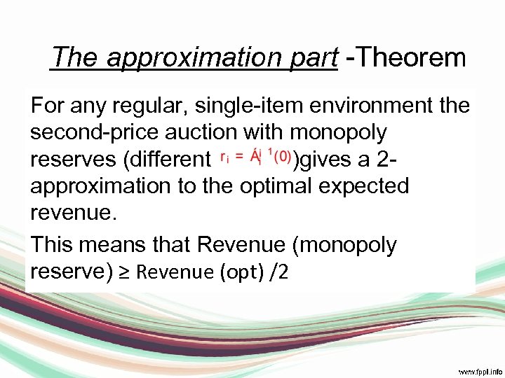The approximation part -Theorem For any regular, single-item environment the second-price auction with monopoly reserves (different )gives a 2 approximation to the optimal expected revenue. This means that Revenue (monopoly reserve) ≥ Revenue (opt) /2

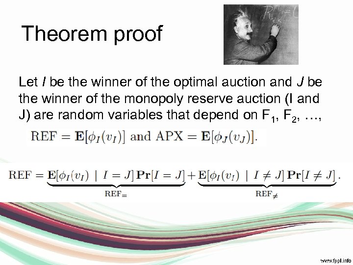Theorem proof Let I be the winner of the optimal auction and J be the winner of the monopoly reserve auction (I and J) are random variables that depend on F 1, F 2, …,

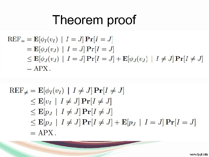Theorem proof

Irregular Distributions • An agent whose value is above the monopoly price may yet have a negative virtual value. • We will show that the regularity property is crucial to the previous Theorem. • Discuss prophet inequalities from optimal stopping theory

Give example that monopoly reserves are bad For irregular distributions (unlike regular distributions). (The “Sydney Opera House example” gives an irregular Distribution for which, EVEN IDENTICALLY DISTRIBUTED Bidders, Even single items, the monopoly reserve price is bad (linear means bad). There are better things to do with irregular distributions: Use ironed virtual prices reserve price or ironed virtual “seqeuential posted price”,

Prophet inequality • We will now talk about a term called prophet inequality. • In order to give a basic idea about this term we will use the Gambler example.

The Gambler example • A gambler faces a series of n games on each of n days. • Game i has prize distributed according to Fi • The order of the games and distribution of the game prizes is fully known in advance to the gambler. • On day i the gambler realizes the value vi ~ Fi of game i and must decide whether to keep this prize and stop or to return the prize and continue playing. • In other words, the gambler is only allowed to keep one prize and must decide which prize to keep immediately on realizing the prize and before any other prizes are realized.

backwards induction • The gambler’s optimal strategy can be calculated by backwards induction. • The gambler last day is his last chance of taking the prize. • The gambler choose to take the prize in the (n-1) day only if the prize value is bigger than in the nth day, and so on (backwards).

backwards induction Strategy disadvantages • It takes n numbers to describe it. • It is not robust to small changes in , the game, such as, changing of the order of the games or making small changes to distribution. • It does not allow for any intuitive understanding of the properties of good strategies. Theorem 4. 7

The connection between the auction problem and the gambler’s problem • the gambler’s problem in prize space is similar to the auctioneer’s problem in ironed-virtualvalue space. • The gambler aims to maximize expected prize while the auctioneer aims to maximize expected virtual value.

uniform ironed virtual price A uniform ironed virtual price is a vector p = (p 1, . . . , pn ) such that for all i and i′: ¯φi(pi) = ¯φi′(pi′).

• For any independent, single-item environment the second-price auction with a uniform ironed virtual reserve price is a 2 -approximation to the optimal auction revenue.

• For any independent, single-item environment a sequential posted pricing of uniform ironed virtual prices is a 2 approximation to the optimal auction revenue.