Semantical and Algorithmic Aspects of the Living François

Semantical and Algorithmic Aspects of the Living François Fages Constraint Programming project-team, INRIA Paris-Rocquencourt To tackle the complexity of biological systems, investigate • Programming Theory Concepts • Formal Methods of Circuit and Program Verification • Automated Reasoning Tools Prototype Implementation in the Biochemical Abstract Machine BIOCHAM modeling environment available at http: //contraintes. inria. fr/BIOCHAM François Fages Rocquencourt, Sep. 2007

Systems Biology ? “Systems Biology aims at systems-level understanding [which] requires a set of principles and methodologies that links the behaviors of molecules to systems characteristics and functions. ” H. Kitano, ICSB 2000 • Analyze (post-)genomic data produced with high-throughput technologies (stored in databases like GO, KEGG, Bio. Cyc, etc. ); • Integrate heterogeneous data about a specific problem; • Understand Predict behaviors or interactions in large networks of genes and proteins. Systems Biology Markup Language (SBML) : exchange format for reaction models François Fages Rocquencourt, Sep. 2007

Issue of Abstraction Models are built in Systems Biology with two contradictory perspectives : François Fages Rocquencourt, Sep. 2007

Issue of Abstraction Models are built in Systems Biology with two contradictory perspectives : 1) Models for representing knowledge : the more concrete the better François Fages Rocquencourt, Sep. 2007

Issue of Abstraction Models are built in Systems Biology with two contradictory perspectives : 1) Models for representing knowledge : the more concrete the better 2) Models for making predictions : the more abstract the better ! François Fages Rocquencourt, Sep. 2007

Issue of Abstraction Models are built in Systems Biology with two contradictory perspectives : 1) Models for representing knowledge : the more concrete the better 2) Models for making predictions : the more abstract the better ! These perspectives can be reconciled by organizing formalisms and models into hierarchies of abstractions. To understand a system is not to know everything about it but to know abstraction levels that are sufficient for answering questions about it François Fages Rocquencourt, Sep. 2007

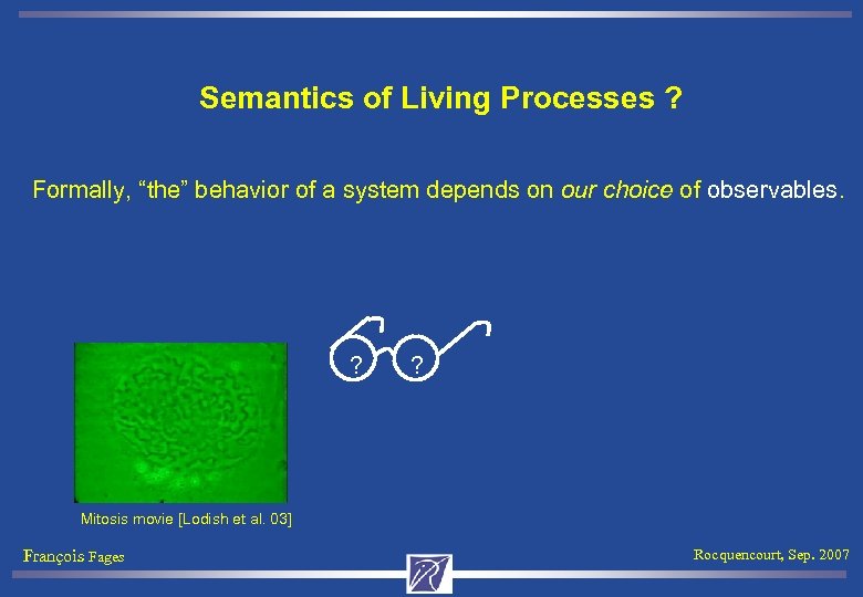Semantics of Living Processes ? Formally, “the” behavior of a system depends on our choice of observables. ? ? Mitosis movie [Lodish et al. 03] François Fages Rocquencourt, Sep. 2007

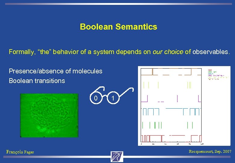Boolean Semantics Formally, “the” behavior of a system depends on our choice of observables. Presence/absence of molecules Boolean transitions 0 François Fages 1 Rocquencourt, Sep. 2007

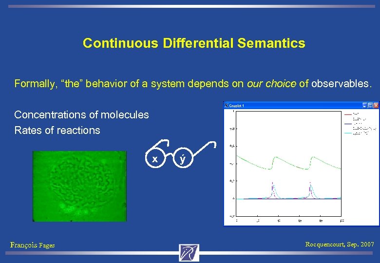Continuous Differential Semantics Formally, “the” behavior of a system depends on our choice of observables. Concentrations of molecules Rates of reactions x François Fages ý Rocquencourt, Sep. 2007

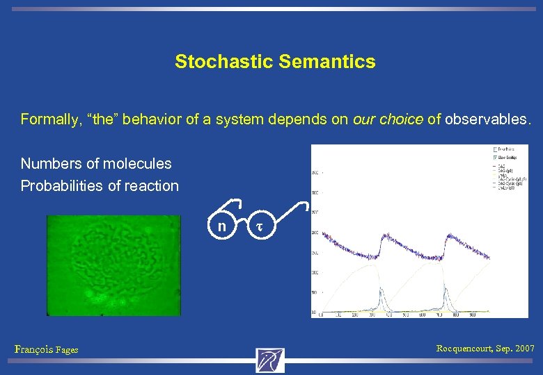Stochastic Semantics Formally, “the” behavior of a system depends on our choice of observables. Numbers of molecules Probabilities of reaction n François Fages Rocquencourt, Sep. 2007

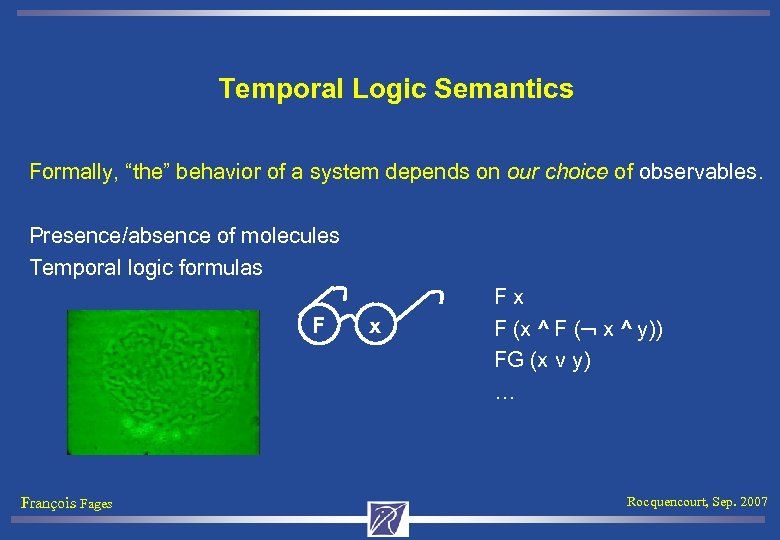Temporal Logic Semantics Formally, “the” behavior of a system depends on our choice of observables. Presence/absence of molecules Temporal logic formulas F François Fages x F (x ^ F ( x ^ y)) FG (x v y) … Rocquencourt, Sep. 2007

Constraint Temporal Logic Semantics Formally, “the” behavior of a system depends on our choice of observables. Concentrations of molecules Constraint LTL temporal formulas F François Fages x>1 F (x >0. 2) F (x >0. 2 ^ F (x<0. 1 ^ y>0. 2)) FG (x>0. 2 v y>0. 2) … Rocquencourt, Sep. 2007

Language-based Approaches to Cell Systems Biology Qualitative models: from diagrammatic notation to • Boolean networks [Kaufman 69, Thomas 73] • Petri Nets [Reddy 93, Chaouiya 05] • Process algebra π–calculus [Regev-Silverman-Shapiro 99 -01, Nagasali et al. 00] • Bio-ambients [Regev-Panina-Silverman-Cardelli-Shapiro 03] • Pathway logic [Eker-Knapp-Laderoute-Lincoln-Meseguer-Sonmez 02] • Reaction rules [Chabrier-Fages 03] [Chabrier-Chiaverini-Danos-Fages-Schachter 04] Quantitative models: from ODEs and stochastic simulations to • Hybrid Petri nets [Hofestadt-Thelen 98, Matsuno et al. 00] • Hybrid automata [Alur et al. 01, Ghosh-Tomlin 01] HCC [Bockmayr-Courtois 01] • Stochastic π–calculus [Priami et al. 03] [Cardelli et al. 06] • Reaction rules with continuous time dynamics [Fages-Soliman-Chabrier 04] François Fages Rocquencourt, Sep. 2007

Overview of the Talk 1. Rule-based Modeling of Biochemical Systems 1. Syntax of molecules, compartments and reactions 2. Semantics at three abstraction levels: boolean, differential, stochastic 3. Cell cycle control models 2. Temporal Logic Language for Formalizing Biological Properties 1. CTL for the boolean semantics 2. Constraint LTL for the differential semantics 3. PCTL for the stochastic semantics 3. Automated Reasoning Tools 1. Inferring kinetic parameter values from Constraint-LTL specification 2. Inferring reaction rules from CTL specification L. Calzone, N. Chabrier, F. Fages, S. Soliman. TCSB VI, LNBI 4220: 68 -94. 2006. François Fages Rocquencourt, Sep. 2007

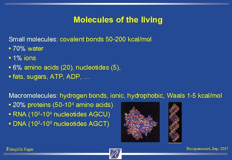Molecules of the living Small molecules: covalent bonds 50 -200 kcal/mol • 70% water • 1% ions • 6% amino acids (20), nucleotides (5), • fats, sugars, ATP, ADP, … Macromolecules: hydrogen bonds, ionic, hydrophobic, Waals 1 -5 kcal/mol • 20% proteins (50 -104 amino acids) • RNA (102 -104 nucleotides AGCU) • DNA (102 -106 nucleotides AGCT) François Fages Rocquencourt, Sep. 2007

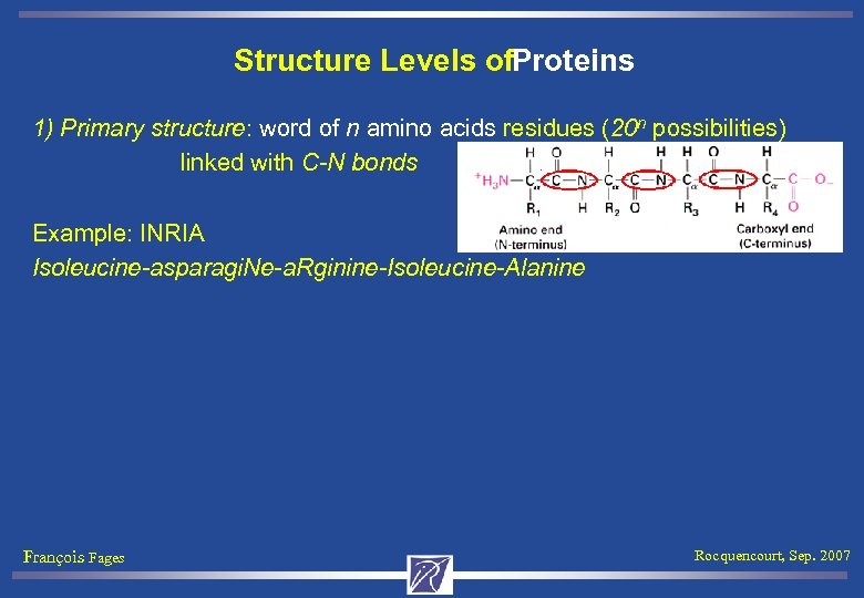Structure Levels of. Proteins 1) Primary structure: word of n amino acids residues (20 n possibilities) linked with C-N bonds Example: INRIA Isoleucine-asparagi. Ne-a. Rginine-Isoleucine-Alanine François Fages Rocquencourt, Sep. 2007

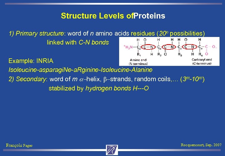Structure Levels of. Proteins 1) Primary structure: word of n amino acids residues (20 n possibilities) linked with C-N bonds Example: INRIA Isoleucine-asparagi. Ne-a. Rginine-Isoleucine-Alanine 2) Secondary: word of m a-helix, b-strands, random coils, … (3 m-10 m) stabilized by hydrogen bonds H---O François Fages Rocquencourt, Sep. 2007

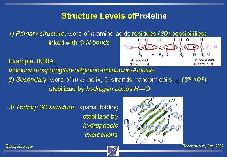Structure Levels of. Proteins 1) Primary structure: word of n amino acids residues (20 n possibilities) linked with C-N bonds Example: INRIA Isoleucine-asparagi. Ne-a. Rginine-Isoleucine-Alanine 2) Secondary: word of m a-helix, b-strands, random coils, … (3 m-10 m) stabilized by hydrogen bonds H---O 3) Tertiary 3 D structure: spatial folding stabilized by hydrophobic interactions François Fages Rocquencourt, Sep. 2007

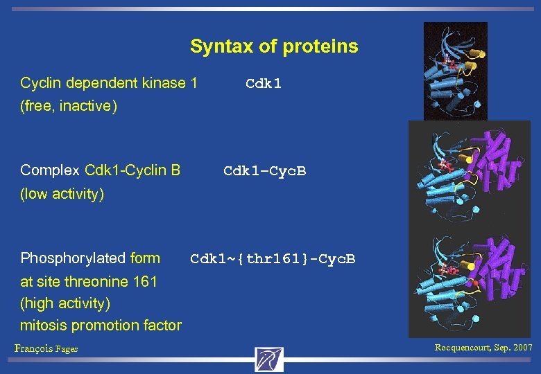Syntax of proteins Cyclin dependent kinase 1 Cdk 1 (free, inactive) Complex Cdk 1 -Cyclin B Cdk 1–Cyc. B (low activity) Phosphorylated form Cdk 1~{thr 161}-Cyc. B at site threonine 161 (high activity) mitosis promotion factor François Fages Rocquencourt, Sep. 2007

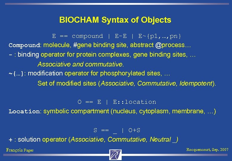BIOCHAM Syntax of Objects E == compound | E-E | E~{p 1, …, pn} Compound: molecule, #gene binding site, abstract @process… - : binding operator for protein complexes, gene binding sites, … Associative and commutative. ~{…}: modification operator for phosphorylated sites, … Set of modified sites (Associative, Commutative, Idempotent). O == E | E: : location Location: symbolic compartment (nucleus, cytoplasm, membrane, …) S == _ | O+S + : solution operator (Associative, Commutative, Neutral _) François Fages Rocquencourt, Sep. 2007

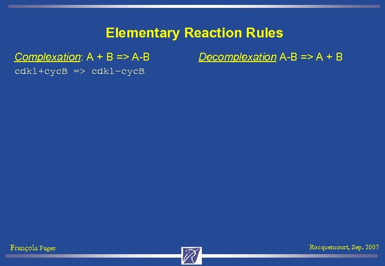Elementary Reaction Rules Complexation: A + B => A-B Decomplexation A-B => A + B cdk 1+cyc. B => cdk 1–cyc. B François Fages Rocquencourt, Sep. 2007

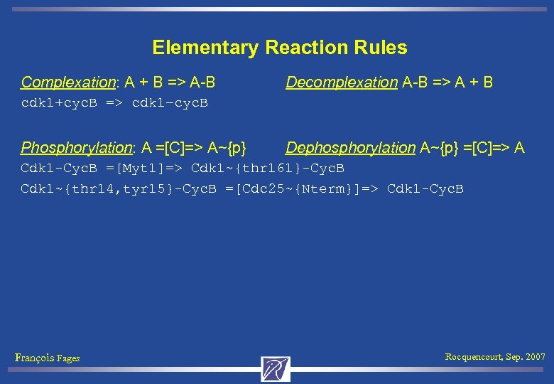Elementary Reaction Rules Complexation: A + B => A-B Decomplexation A-B => A + B cdk 1+cyc. B => cdk 1–cyc. B Phosphorylation: A =[C]=> A~{p} Dephosphorylation A~{p} =[C]=> A Cdk 1 -Cyc. B =[Myt 1]=> Cdk 1~{thr 161}-Cyc. B Cdk 1~{thr 14, tyr 15}-Cyc. B =[Cdc 25~{Nterm}]=> Cdk 1 -Cyc. B François Fages Rocquencourt, Sep. 2007

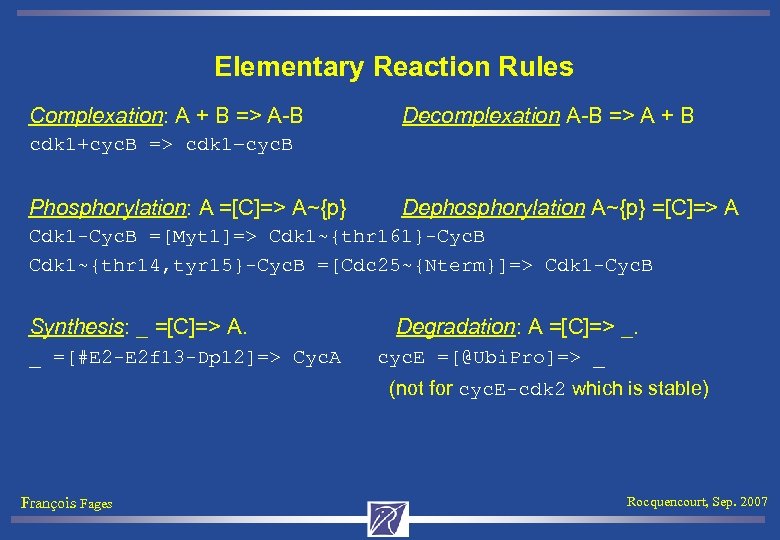Elementary Reaction Rules Complexation: A + B => A-B Decomplexation A-B => A + B cdk 1+cyc. B => cdk 1–cyc. B Phosphorylation: A =[C]=> A~{p} Dephosphorylation A~{p} =[C]=> A Cdk 1 -Cyc. B =[Myt 1]=> Cdk 1~{thr 161}-Cyc. B Cdk 1~{thr 14, tyr 15}-Cyc. B =[Cdc 25~{Nterm}]=> Cdk 1 -Cyc. B Synthesis: _ =[C]=> A. Degradation: A =[C]=> _. _ =[#E 2 -E 2 f 13 -Dp 12]=> Cyc. A cyc. E =[@Ubi. Pro]=> _ (not for cyc. E-cdk 2 which is stable) François Fages Rocquencourt, Sep. 2007

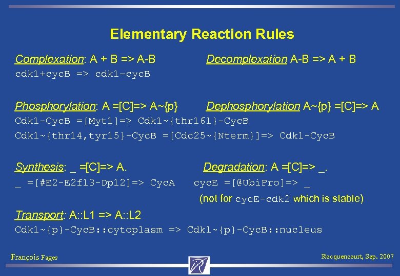Elementary Reaction Rules Complexation: A + B => A-B Decomplexation A-B => A + B cdk 1+cyc. B => cdk 1–cyc. B Phosphorylation: A =[C]=> A~{p} Dephosphorylation A~{p} =[C]=> A Cdk 1 -Cyc. B =[Myt 1]=> Cdk 1~{thr 161}-Cyc. B Cdk 1~{thr 14, tyr 15}-Cyc. B =[Cdc 25~{Nterm}]=> Cdk 1 -Cyc. B Synthesis: _ =[C]=> A. Degradation: A =[C]=> _. _ =[#E 2 -E 2 f 13 -Dp 12]=> Cyc. A cyc. E =[@Ubi. Pro]=> _ (not for cyc. E-cdk 2 which is stable) Transport: A: : L 1 => A: : L 2 Cdk 1~{p}-Cyc. B: : cytoplasm => Cdk 1~{p}-Cyc. B: : nucleus François Fages Rocquencourt, Sep. 2007

From Syntax to Semantics R : : = S=>S | S =[O]=> S | S <=[O]=> S where A =[C]=> B stands for A+C => B+C A <=> B stands for A=>B and B=>A, etc. | kinetic for R (import/export SBML format) In SBML : no semantics (exchange format) François Fages Rocquencourt, Sep. 2007

From Syntax to Semantics R : : = S=>S | S =[O]=> S | S <=[O]=> S where A =[C]=> B stands for A+C => B+C A <=> B stands for A=>B and B=>A, etc. | kinetic for R (import/export SBML format) In SBML : no semantics (exchange format) In BIOCHAM : three abstraction levels 1. Boolean Semantics: presence-absence of molecules 1. Concurrent Transition System (asynchronous, non-deterministic) François Fages Rocquencourt, Sep. 2007

From Syntax to Semantics R : : = S=>S | S =[O]=> S | S <=[O]=> S where A =[C]=> B stands for A+C => B+C A <=> B stands for A=>B and B=>A, etc. | kinetic for R (import/export SBML format) In SBML : no semantics (exchange format) In BIOCHAM : three abstraction levels 1. Boolean Semantics: presence-absence of molecules 1. Concurrent Transition System (asynchronous, non-deterministic) 2. Differential Semantics: concentration • Ordinary Differential Equations or Hybrid system (deterministic) François Fages Rocquencourt, Sep. 2007

From Syntax to Semantics R : : = S=>S | S =[O]=> S | S <=[O]=> S where A =[C]=> B stands for A+C => B+C A <=> B stands for A=>B and B=>A, etc. | kinetic for R (import/export SBML format) In SBML : no semantics (exchange format) In BIOCHAM : three abstraction levels 1. Boolean Semantics: presence-absence of molecules 1. Concurrent Transition System (asynchronous, non-deterministic) 2. Differential Semantics: concentration 1. Ordinary Differential Equations or Hybrid system (deterministic) • Stochastic Semantics: number of molecules • Continuous time Markov chain François Fages Rocquencourt, Sep. 2007

1. Differential Semantics Associates to each molecule its concentration [Ai]= | Ai| / volume ML-1 volume of diffusion … François Fages Rocquencourt, Sep. 2007

1. Differential Semantics Associates to each molecule its concentration [Ai]= | Ai| / volume ML-1 volume of compartment Compiles a set of rules { ei for Si=>S’I }i=1, …, n (by default ei is MA(1)) into the system of ODEs (or hybrid automaton) over variables {A 1, …, Ak} d. A/dt = Σni=1 ri(A)*ei - Σnj=1 lj(A)*ej where ri(A) (resp. li(A)) is the stoichiometric coefficient of A in Si (resp. S’i) multiplied by the volume ratio of the location of A. François Fages Rocquencourt, Sep. 2007

1. Differential Semantics Associates to each molecule its concentration [Ai]= | Ai| / volume ML-1 volume of compartment Compiles a set of rules { ei for Si=>S’I }i=1, …, n (by default ei is MA(1)) into the system of ODEs (or hybrid automaton) over variables {A 1, …, Ak} d. A/dt = Σni=1 ri(A)*ei - Σnj=1 lj(A)*ej where ri(A) (resp. li(A)) is the stoichiometric coefficient of A in Si (resp. S’i) multiplied by the volume ratio of the location of A. volume_ratio (15, n), (1, c). m. RNAcyc. A: : n <=> m. RNAcyc. A: : c. means 15*Vn = Vc and is equivalent to 15*m. RNAcyc. A: : n <=> m. RNAcyc. A: : c. François Fages Rocquencourt, Sep. 2007

Numerical Integration • Adaptive step size 4 th order Runge-Kutta can be weak for stiff systems • Rosenbrock implicit method using the Jacobian matrix ∂x’i/∂xj computes a (clever) discretization of time and a time series of concentrations and their derivatives (t 0, X 0, d. X 0/dt), (t 1, X 1, d. X 1/dt), …, (tn, Xn, d. Xn/dt), … at discrete time points François Fages Rocquencourt, Sep. 2007

2. Stochastic Semantics Associate to each molecule its number |Ai| in its location of volume Vi François Fages Rocquencourt, Sep. 2007

2. Stochastic Semantics Associate to each molecule its number |Ai| in its location of volume Vi Compile the rule set into a continuous time Markov chain over vector states X=(|A 1|, …, |Ak|) and where the transition rate τi for the reaction ei for Si=>S’I (giving probability after normalization) is obtained from ei by replacing concentrations by molecule numbers François Fages Rocquencourt, Sep. 2007

2. Stochastic Semantics Associate to each molecule its number |Ai| in its location of volume Vi Compile the rule set into a continuous time Markov chain over vector states X=(|A 1|, …, |Ak|) and where the transition rate τi for the reaction ei for Si=>S’I (giving probability after normalization) is obtained from ei by replacing concentrations by molecule numbers Stochastic simulation [Gillespie 76, Gibson 00] computes realizations as time series (t 0, X 0), (t 1, X 1), …, (tn, Xn), … François Fages Rocquencourt, Sep. 2007

3. Boolean Semantics Associate to each molecule a Boolean denoting its presence/absence in its location François Fages Rocquencourt, Sep. 2007

3. Boolean Semantics Associate to each molecule a Boolean denoting its presence/absence in its location Compile the rule set into an asynchronous transition system François Fages Rocquencourt, Sep. 2007

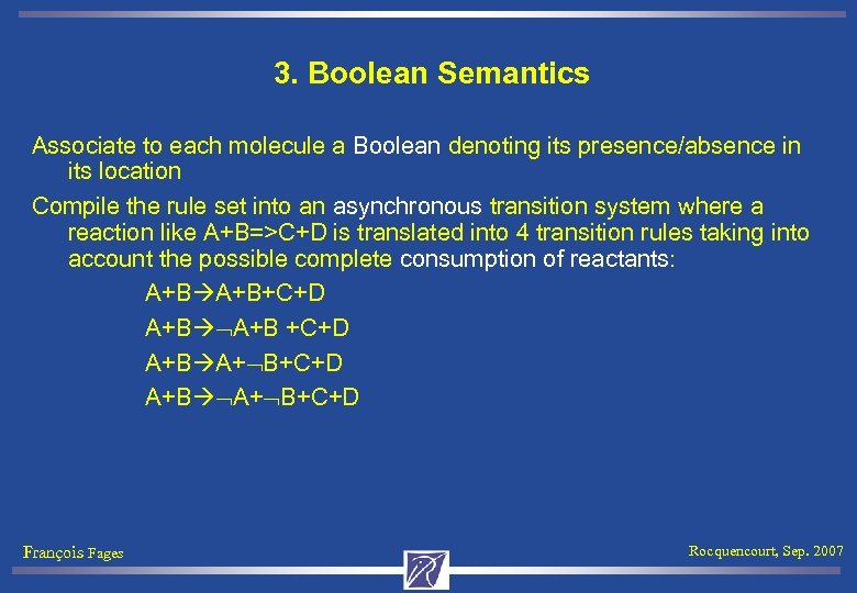3. Boolean Semantics Associate to each molecule a Boolean denoting its presence/absence in its location Compile the rule set into an asynchronous transition system where a reaction like A+B=>C+D is translated into 4 transition rules taking into account the possible complete consumption of reactants: A+B+C+D A+B +C+D A+B A+ B+C+D François Fages Rocquencourt, Sep. 2007

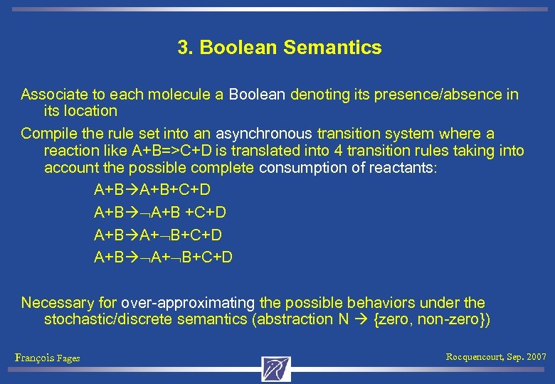3. Boolean Semantics Associate to each molecule a Boolean denoting its presence/absence in its location Compile the rule set into an asynchronous transition system where a reaction like A+B=>C+D is translated into 4 transition rules taking into account the possible complete consumption of reactants: A+B+C+D A+B +C+D A+B A+ B+C+D Necessary for over-approximating the possible behaviors under the stochastic/discrete semantics (abstraction N {zero, non-zero}) François Fages Rocquencourt, Sep. 2007

Hierarchy of Semantics abstraction Boolean model Theory of abstract Interpretation [Cousot POPL’ 77] [Fages Soliman TCSc’ 07] Discrete model Differential model Stochastic model concretization François Fages Syntactical model Models for answering queries: The more abstract the better Optimal abstraction w. r. t. query Rocquencourt, Sep. 2007

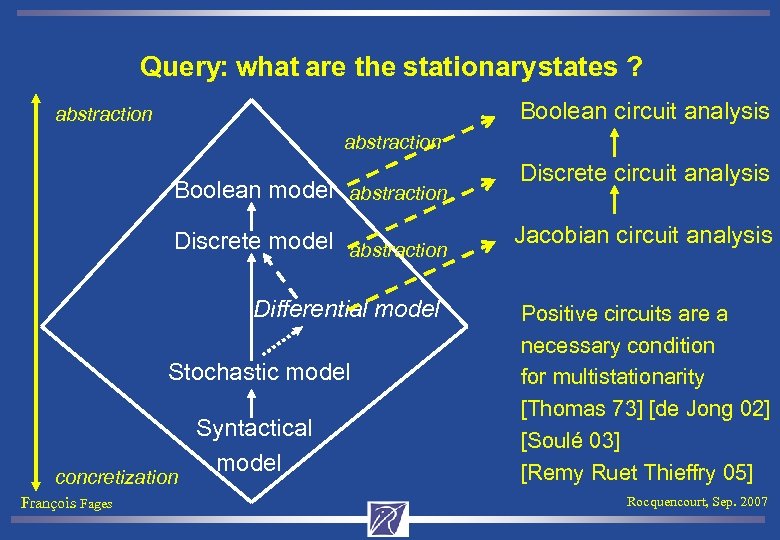Query: what are the stationary states ? Boolean circuit analysis abstraction Boolean model abstraction Discrete model abstraction Differential model Stochastic model concretization François Fages Syntactical model Discrete circuit analysis Jacobian circuit analysis Positive circuits are a necessary condition for multistationarity [Thomas 73] [de Jong 02] [Soulé 03] [Remy Ruet Thieffry 05] Rocquencourt, Sep. 2007

Type Inference / Type Checking abstraction [Fages Soliman CMSB’ 06] Boolean model Discrete model Differential model Influence graph of proteins Stochastic model concretization François Fages Syntactical model Protein functions (kinase, phosphatase, …) Compartments topology Rocquencourt, Sep. 2007

Type Inference / Type Checking abstraction [Fages Soliman CMSB’ 06] Boolean model Discrete model Influence graph of proteins (activation/inhibition) Differential model Influence graph of proteins Stochastic model concretization François Fages Syntactical model Protein functions (kinase, phosphatase, …) Compartments topology Rocquencourt, Sep. 2007

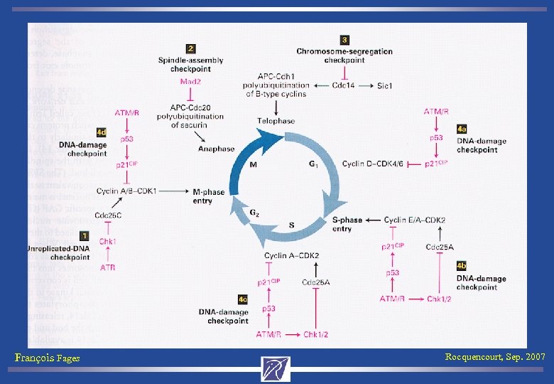
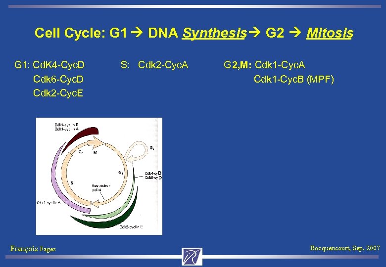Cell Cycle: G 1 DNA Synthesis G 2 Mitosis G 1: Cd. K 4 -Cyc. D S: Cdk 2 -Cyc. A G 2, M: Cdk 1 -Cyc. A Cdk 6 -Cyc. D Cdk 1 -Cyc. B (MPF) Cdk 2 -Cyc. E François Fages Rocquencourt, Sep. 2007

Example: Cell Cycle Control Model Tyson 91] [ MA(k 1) for MA(k 2) for MA(K 7) for _ => Cyclin => _. Cyclin~{p 1} => _. MA(k 8) for MA(k 9) for Cdc 2 => Cdc 2~{p 1} =>Cdc 2. MA(k 3) for Cyclin+Cdc 2~{p 1} => Cdc 2~{p 1}-Cyclin~{p 1}. MA(k 4 p) for Cdc 2~{p 1}-Cyclin~{p 1} => Cdc 2 -Cyclin~{p 1}. k 4*[Cdc 2 -Cyclin~{p 1}]^2*[Cdc 2~{p 1}-Cyclin~{p 1}] for Cdc 2~{p 1}-Cyclin~{p 1} =[Cdc 2 -Cyclin~{p 1}] => Cdc 2 -Cyclin~{p 1}. MA(k 5) for Cdc 2 -Cyclin~{p 1} => Cdc 2~{p 1}-Cyclin~{p 1}. MA(k 6) for Cdc 2 -Cyclin~{p 1} => Cdc 2+Cyclin~{p 1}. François Fages Rocquencourt, Sep. 2007

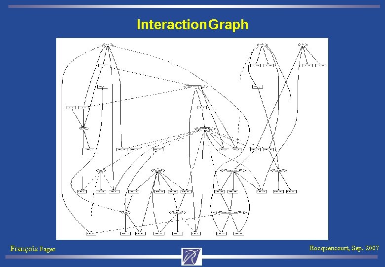Interaction Graph François Fages Rocquencourt, Sep. 2007

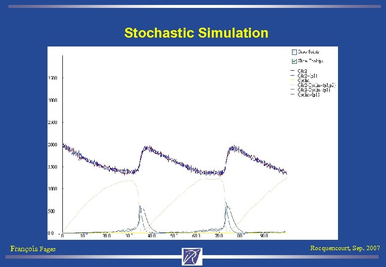Stochastic Simulation François Fages Rocquencourt, Sep. 2007

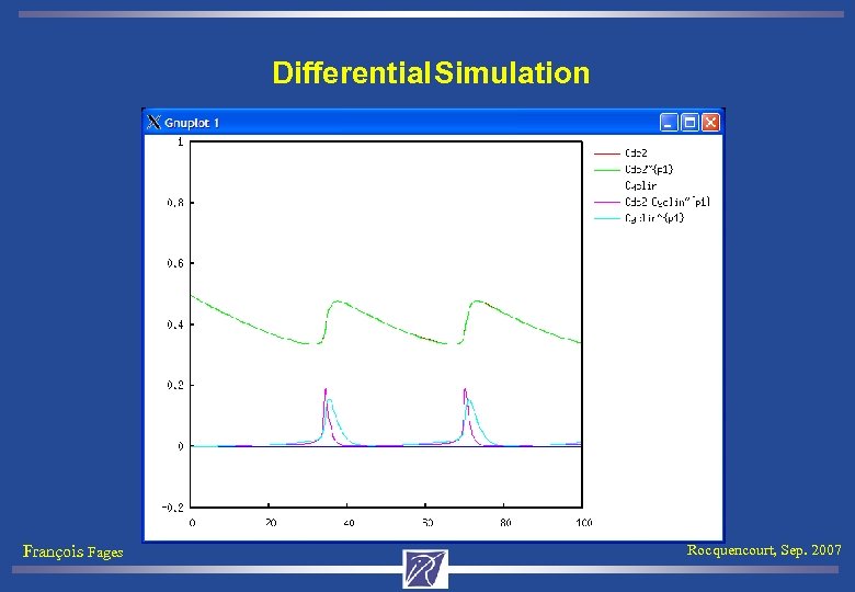Differential Simulation François Fages Rocquencourt, Sep. 2007

Boolean Simulation François Fages Rocquencourt, Sep. 2007

François Fages Rocquencourt, Sep. 2007

Mammalian Cell Cycle Control. Map [Kohn 99] François Fages Rocquencourt, Sep. 2007

Transcriptionof Kohn’s Map _ =[ E 2 F 13 -DP 12 -g. E 2 ]=> cyc. A. . cyc. B =[ APC~{p 1} ]=>_. cdk 1~{p 1, p 2, p 3} + cyc. A => cdk 1~{p 1, p 2, p 3}-cyc. A. cdk 1~{p 1, p 2, p 3} + cyc. B => cdk 1~{p 1, p 2, p 3}-cyc. B. . cdk 1~{p 1, p 3}-cyc. A =[ Wee 1 ]=> cdk 1~{p 1, p 2, p 3}-cyc. A. cdk 1~{p 1, p 3}-cyc. B =[ Wee 1 ]=> cdk 1~{p 1, p 2, p 3}-cyc. B. cdk 1~{p 2, p 3}-cyc. A =[ Myt 1 ]=> cdk 1~{p 1, p 2, p 3}-cyc. A. cdk 1~{p 2, p 3}-cyc. B =[ Myt 1 ]=> cdk 1~{p 1, p 2, p 3}-cyc. B. . cdk 1~{p 1, p 2, p 3} =[ cdc 25 C~{p 1, p 2} ]=> cdk 1~{p 1, p 3}. cdk 1~{p 1, p 2, p 3}-cyc. A =[ cdc 25 C~{p 1, p 2} ]=> cdk 1~{p 1, p 3}-cyc. A. cdk 1~{p 1, p 2, p 3}-cyc. B =[ cdc 25 C~{p 1, p 2} ]=> cdk 1~{p 1, p 3}-cyc. B. 165 proteins and genes, 500 variables, 800 rules [Chiaverini Danos 02] François Fages Rocquencourt, Sep. 2007

Overview of the Talk 1. Rule-based Modeling of Biochemical Systems 1. Syntax of molecules, compartments and reactions 2. Semantics at three abstraction levels: boolean, differential, stochastic 3. Cell cycle control models 2. Temporal Logic Language for Formalizing Biological Properties 1. CTL for the boolean semantics 2. Constraint LTL for the differential semantics 3. PCTL for the stochastic semantics 3. Automated Reasoning Tools 1. Inferring kinetic parameter values from Constraint-LTL specification 2. Inferring reaction rules from CTL specification François Fages Rocquencourt, Sep. 2007

A Logical Paradigm for Systems Biology Biological model = Transition System Biological property = Temporal Logic Formula Biological validation = Model-checking Formalize properties of the biological system in: • Computation Tree Logic CTL for the boolean semantics • Linear Time Logic with numerical constraints for the concentration semantics • Probabilistic CTL with numerical constraints for the stochastic semantics Evaluate the formulas by model checking techniques [Lincoln et al. PSB’ 02] [Chabrier Fages CMSB’ 03] [Bernot et al. TCS’ 04] … François Fages Rocquencourt, Sep. 2007

A Logical Paradigm for Systems Biology Biological model = Transition System Biological property = Temporal Logic Formula Biological validation = Model-checking In the Biochemical Abstract Machine environment, Model: BIOCHAM - Boolean - simulation - Differential - Stochastic (SBML) François Fages Rocquencourt, Sep. 2007

A Logical Paradigm for Systems Biology Biological model = Transition System Biological property = Temporal Logic Formula Biological validation = Model-checking In the Biochemical Abstract Machine environment, Model: BIOCHAM Biological Properties: - Boolean - simulation - CTL - Differential - query evaluation - LTL with constraints - Stochastic - PCTL with constraints (SBML) François Fages Rocquencourt, Sep. 2007

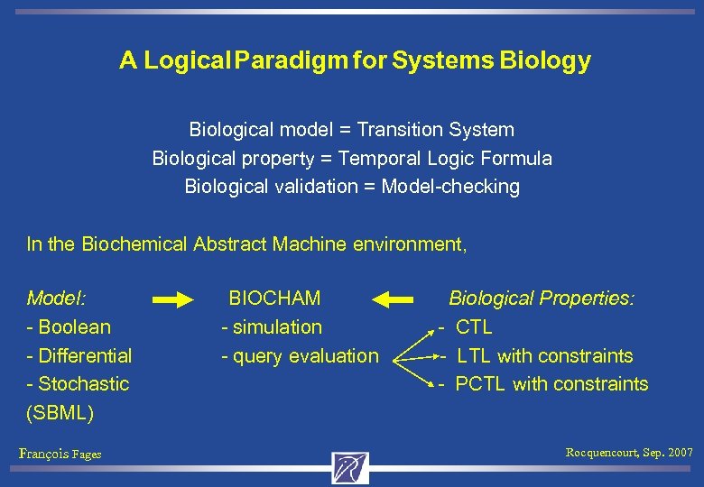A Logical Paradigm for Systems Biology Biological model = Transition System Biological property = Temporal Logic Formula Biological validation = Model-checking In the Biochemical Abstract Machine environment, Model: BIOCHAM Biological Properties: - Boolean - simulation - CTL - Differential - query evaluation - LTL with constraints - Stochastic - PCTL with constraints (SBML) François Fages Rocquencourt, Sep. 2007

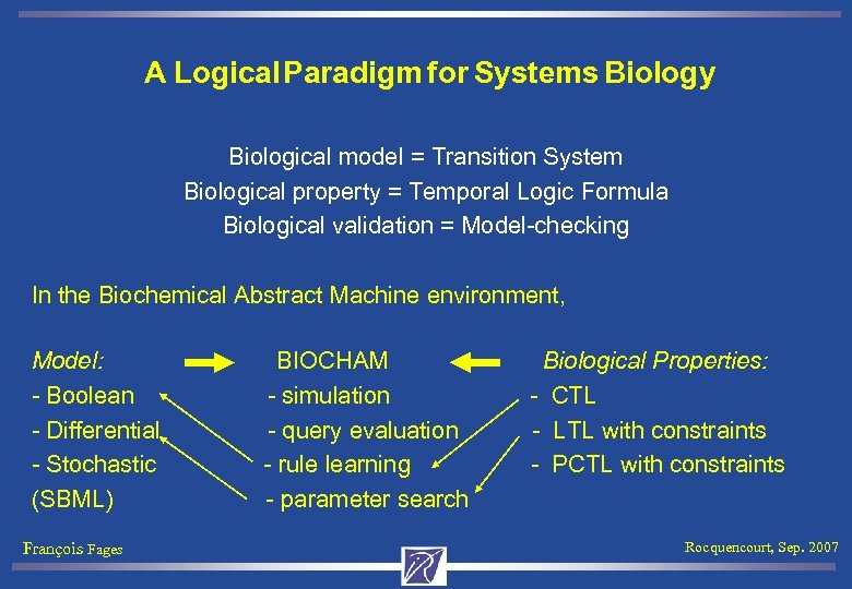A Logical Paradigm for Systems Biology Biological model = Transition System Biological property = Temporal Logic Formula Biological validation = Model-checking In the Biochemical Abstract Machine environment, Model: BIOCHAM Biological Properties: - Boolean - simulation - CTL - Differential - query evaluation - LTL with constraints - Stochastic - rule learning - PCTL with constraints (SBML) - parameter search François Fages Rocquencourt, Sep. 2007

2. 1 Computation Tree Logic CTL Extension of propositional (or first-order) logic with operators for time and choices [Clarke et al. 99] Choice Time E exists A always X next time EX(f) ¬ AX(¬ f) AX(f) F finally EF(f) ¬ AG(¬ f) AF(f) G globally EG(f) ¬ AF(¬ f) AG(f) U until François Fages E (f 1 U f 2) Non-determinism E, A AG A (f 1 U f 2) EU F, G, U Time EF Rocquencourt, Sep. 2007

Biological Properties formalized in CTL (1/3) About reachability: • Can the cell produce some protein P? reachable(P)==EF(P) François Fages Rocquencourt, Sep. 2007

Biological Properties formalized in CTL (1/3) About reachability: • Can the cell produce some protein P? reachable(P)==EF(P) • Can the cell produce P, Q and not R? reachable(P^Q^ R) François Fages Rocquencourt, Sep. 2007

Biological Properties formalized in CTL (1/3) About reachability: • Can the cell produce some protein P? reachable(P)==EF(P) • Can the cell produce P, Q and not R? reachable(P^Q^ R) • Can the cell always produce P? AG(reachable(P)) François Fages Rocquencourt, Sep. 2007

Biological Properties formalized in CTL (1/3) About reachability: • Can the cell produce some protein P? reachable(P)==EF(P) • Can the cell produce P, Q and not R? reachable(P^Q^ R) • Can the cell always produce P? AG(reachable(P)) About pathways: • Can the cell reach a (partially described) set of states s while passing by another set of states s 2? EF(s 2^EFs) François Fages Rocquencourt, Sep. 2007

Biological Properties formalized in CTL (1/3) About reachability: • Can the cell produce some protein P? reachable(P)==EF(P) • Can the cell produce P, Q and not R? reachable(P^Q^ R) • Can the cell always produce P? AG(reachable(P)) About pathways: • Can the cell reach a (partially described) set of states s while passing by another set of states s 2? EF(s 2^EFs) • Is it possible to produce P without Q? E( Q U P) François Fages Rocquencourt, Sep. 2007

Biological Properties formalized in CTL (1/3) About reachability: • Can the cell produce some protein P? reachable(P)==EF(P) • Can the cell produce P, Q and not R? reachable(P^Q^ R) • Can the cell always produce P? AG(reachable(P)) About pathways: • Can the cell reach a (partially described) set of states s while passing by another set of states s 2? EF(s 2^EFs) • Is it possible to produce P without Q? E( Q U P) • Is (set of) state s 2 a necessary checkpoint for reaching (set of) state s? checkpoint(s 2, s)== E( s 2 U s) François Fages Rocquencourt, Sep. 2007

Biological Properties formalized in CTL (1/3) About reachability: • Can the cell produce some protein P? reachable(P)==EF(P) • Can the cell produce P, Q and not R? reachable(P^Q^ R) • Can the cell always produce P? AG(reachable(P)) About pathways: • Can the cell reach a (partially described) set of states s while passing by another set of states s 2? EF(s 2^EFs) • Is it possible to produce P without Q? E( Q U P) • Is (set of) state s 2 a necessary checkpoint for reaching (set of) state s? checkpoint(s 2, s)== E( s 2 U s) • Is s 2 always a checkpoint for s? AG( s -> checkpoint(s 2, s)) François Fages Rocquencourt, Sep. 2007

Biological Properties formalized in CTL (2/3) About stationarity: • Is a (set of) state s a stable state? stable(s)== AG(s) François Fages Rocquencourt, Sep. 2007

Biological Properties formalized in CTL (2/3) About stationarity: • Is a (set of) state s a stable state? stable(s)== AG(s) • Is s a steady state (with possibility of escaping) ? steady(s)==EG(s) François Fages Rocquencourt, Sep. 2007

Biological Properties formalized in CTL (2/3) About stationarity: • Is a (set of) state s a stable state? stable(s)== AG(s) • Is s a steady state (with possibility of escaping) ? steady(s)==EG(s) • Can the cell reach a stable state s? EF(stable(s)) not in LTL François Fages Rocquencourt, Sep. 2007

Biological Properties formalized in CTL (2/3) About stationarity: • Is a (set of) state s a stable state? stable(s)== AG(s) • Is s a steady state (with possibility of escaping) ? steady(s)==EG(s) • Can the cell reach a stable state s? EF(stable(s)) not in LTL • Must the cell reach a stable state s? AG(stable(s)) François Fages Rocquencourt, Sep. 2007

Biological Properties formalized in CTL (2/3) About stationarity: • Is a (set of) state s a stable state? stable(s)== AG(s) • Is s a steady state (with possibility of escaping) ? steady(s)==EG(s) • Can the cell reach a stable state s? EF(stable(s)) not in LTL • Must the cell reach a stable state s? AG(stable(s)) • What are the stable states? Not expressible in CTL. Needs to combine CTL with search (e. g. constraint programming [Thieffry et al. 05] ) François Fages Rocquencourt, Sep. 2007

Biological Properties formalized in CTL (3/3) About oscillations: • Can the system exhibit a cyclic behavior w. r. t. the presence of P ? oscil(P)== EG(F P ^ F P) CTL* formula that can be approximated in CTL by oscil(P)== EG((P EF P) ^ ( P EF P)) (necessary but not sufficient condition for oscillation) François Fages Rocquencourt, Sep. 2007

Biological Properties formalized in CTL (3/3) About oscillations: • Can the system exhibit a cyclic behavior w. r. t. the presence of P ? oscil(P)== EG((P EF P) ^ ( P EF P)) (necessary but not sufficient condition) • Can the system loops between states s and s 2 ? loop(P, Q)== EG((s EF s 2) ^ (s 2 EF s)) François Fages Rocquencourt, Sep. 2007

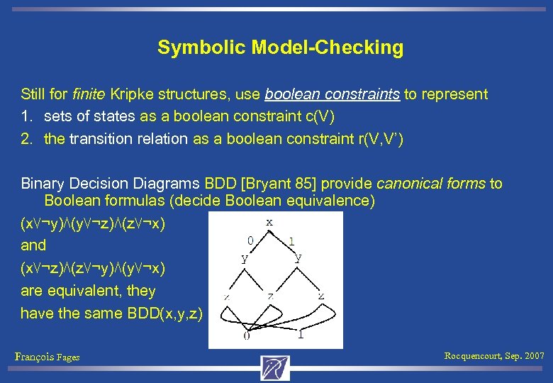Symbolic Model-Checking Still for finite Kripke structures, use boolean constraints to represent 1. sets of states as a boolean constraint c(V) 2. the transition relation as a boolean constraint r(V, V’) Binary Decision Diagrams BDD [Bryant 85] provide canonical forms to Boolean formulas (decide Boolean equivalence) (x⋁¬y)⋀(y⋁¬z)⋀(z⋁¬x) and (x⋁¬z)⋀(z⋁¬y)⋀(y⋁¬x) are equivalent, they have the same BDD(x, y, z) François Fages Rocquencourt, Sep. 2007

Mammalian Cell Cycle Control. Map [Kohn 99] François Fages Rocquencourt, Sep. 2007

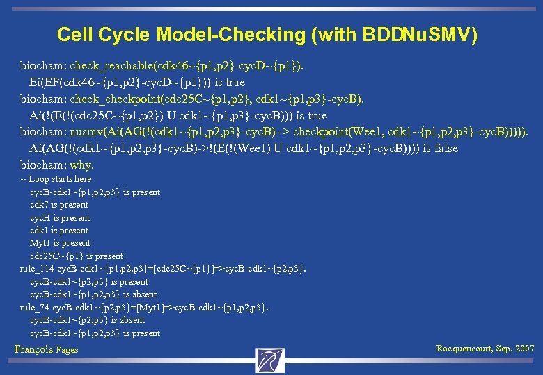Cell Cycle Model-Checking (with BDDNu. SMV) biocham: check_reachable(cdk 46~{p 1, p 2}-cyc. D~{p 1}). Ei(EF(cdk 46~{p 1, p 2}-cyc. D~{p 1})) is true biocham: check_checkpoint(cdc 25 C~{p 1, p 2}, cdk 1~{p 1, p 3}-cyc. B). Ai(!(E(!(cdc 25 C~{p 1, p 2}) U cdk 1~{p 1, p 3}-cyc. B))) is true biocham: nusmv(Ai(AG(!(cdk 1~{p 1, p 2, p 3}-cyc. B) -> checkpoint(Wee 1, cdk 1~{p 1, p 2, p 3}-cyc. B))))). Ai(AG(!(cdk 1~{p 1, p 2, p 3}-cyc. B)->!(E(!(Wee 1) U cdk 1~{p 1, p 2, p 3}-cyc. B)))) is false biocham: why. -- Loop starts here cyc. B-cdk 1~{p 1, p 2, p 3} is present cdk 7 is present cyc. H is present cdk 1 is present Myt 1 is present cdc 25 C~{p 1} is present rule_114 cyc. B-cdk 1~{p 1, p 2, p 3}=[cdc 25 C~{p 1}]=>cyc. B-cdk 1~{p 2, p 3} is present cyc. B-cdk 1~{p 1, p 2, p 3} is absent rule_74 cyc. B-cdk 1~{p 2, p 3}=[Myt 1]=>cyc. B-cdk 1~{p 1, p 2, p 3}. cyc. B-cdk 1~{p 2, p 3} is absent cyc. B-cdk 1~{p 1, p 2, p 3} is present François Fages Rocquencourt, Sep. 2007

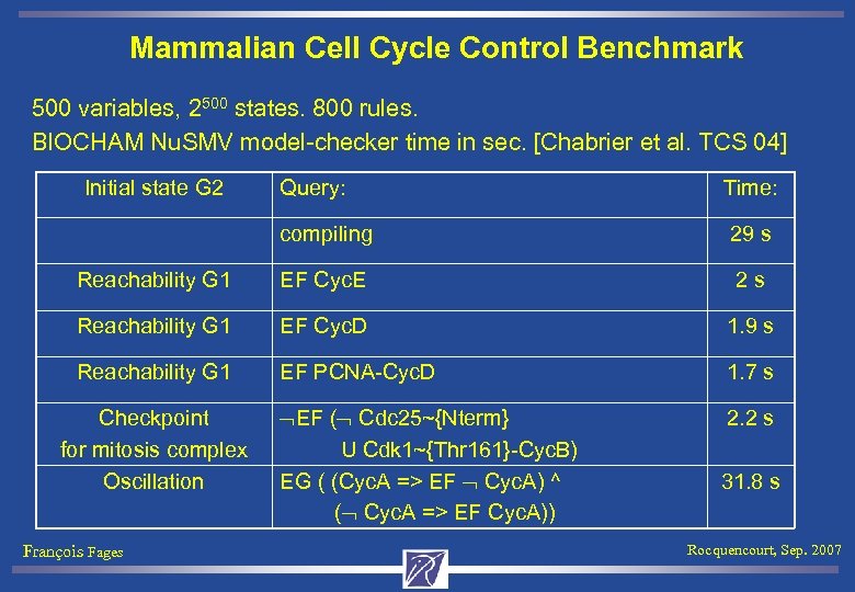Mammalian Cell Cycle Control Benchmark 500 variables, 2500 states. 800 rules. BIOCHAM Nu. SMV model-checker time in sec. [Chabrier et al. TCS 04] Initial state G 2 Query: Time: compiling 29 s Reachability G 1 EF Cyc. E 2 s Reachability G 1 EF Cyc. D 1. 9 s Reachability G 1 EF PCNA-Cyc. D 1. 7 s EF ( Cdc 25~{Nterm} U Cdk 1~{Thr 161}-Cyc. B) EG ( (Cyc. A => EF Cyc. A) ^ ( Cyc. A => EF Cyc. A)) 2. 2 s Checkpoint for mitosis complex Oscillation François Fages 31. 8 s Rocquencourt, Sep. 2007

2. 2 LTL with Constraints for the Differential Semantics • Constraints over concentrations and derivatives as FOL formulae over the reals: • [M] > 0. 2 • [M]+[P] > [Q] • d([M])/dt < 0 François Fages Rocquencourt, Sep. 2007

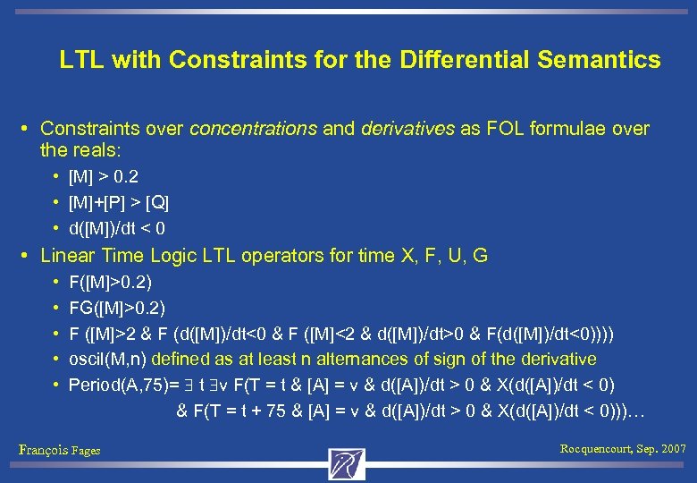LTL with Constraints for the Differential Semantics • Constraints over concentrations and derivatives as FOL formulae over the reals: • [M] > 0. 2 • [M]+[P] > [Q] • d([M])/dt < 0 • Linear Time Logic LTL operators for time X, F, U, G • F([M]>0. 2) • FG([M]>0. 2) • F ([M]>2 & F (d([M])/dt<0 & F ([M]<2 & d([M])/dt>0 & F(d([M])/dt<0)))) • oscil(M, n) defined as at least n alternances of sign of the derivative • Period(A, 75)= t v F(T = t & [A] = v & d([A])/dt > 0 & X(d([A])/dt < 0) & F(T = t + 75 & [A] = v & d([A])/dt > 0 & X(d([A])/dt < 0)))… François Fages Rocquencourt, Sep. 2007

How to Evaluate a Constraint LTL Formula ? • Consider the ODE’s of the concentration semantics d. X/dt = f(X) François Fages Rocquencourt, Sep. 2007

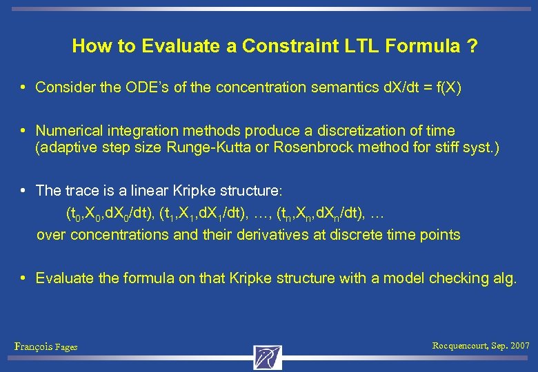How to Evaluate a Constraint LTL Formula ? • Consider the ODE’s of the concentration semantics d. X/dt = f(X) • Numerical integration methods produce a discretization of time (adaptive step size Runge-Kutta or Rosenbrock method for stiff syst. ) • The trace is a linear Kripke structure: (t 0, X 0, d. X 0/dt), (t 1, X 1, d. X 1/dt), …, (tn, Xn, d. Xn/dt), … over concentrations and their derivatives at discrete time points • Evaluate the formula on that Kripke structure with a model checking alg. François Fages Rocquencourt, Sep. 2007

Simulation-Based Constraint LTL Model Checking Hypothesis 1: the initial state is completely known Hypothesis 2: the formula can be checked over a finite period of time [0, T] 1. Run the numerical integration from 0 to T producing values at a finite sequence of time points 2. Iteratively label the time points with the sub-formulae of f that are true: Add f to the time points where a FOL formula f is true, Add F f (X f) to the (immediate) previous time points labeled by f, Add f 1 U f 2 to the predecessor time points of f 2 while they satisfy f 1, (Add G f to the states satisfying f until T) Model checker and numerical integration methods implemented in Prolog François Fages Rocquencourt, Sep. 2007

Constraint-LTLInstanciation. Algo. [Fages Rizk CMSB’ 07] François Fages Rocquencourt, Sep. 2007

2. 3 PCTL Model Checker for the Stochastic Semantics Compute the probability of realisation of a TL formula (with constraints) by Monte Carlo method Perform several stochastic simulations Evaluate the probability of realization of the TL formula Costly… PRISM [Kwiatkowska et al. 04] : PCTL model checker based on BDDs or using Monte Carlo method. François Fages Rocquencourt, Sep. 2007

Overview of the Talk 1. Rule-based Modeling of Biochemical Systems 1. Syntax of molecules, compartments and reactions 2. Semantics at three abstraction levels: boolean, differential, stochastic 3. Cell cycle control models 2. Temporal Logic Language for Formalizing Biological Properties 1. CTL for the boolean semantics 2. Constraint LTL for the differential semantics 3. PCTL for the stochastic semantics 3. Automated Reasoning Tools 1. Inferring kinetic parameter values from Constraint-LTL specification 2. Inferring reaction rules from CTL specification François Fages Rocquencourt, Sep. 2007

Example: Cell Cycle Control Model Tyson 91] [ MA(k 1) for MA(k 2) for MA(K 7) for _ => Cyclin => _. Cyclin~{p 1} => _. MA(k 8) for MA(k 9) for Cdc 2 => Cdc 2~{p 1} =>Cdc 2. MA(k 3) for Cyclin+Cdc 2~{p 1} => Cdc 2~{p 1}-Cyclin~{p 1}. MA(k 4 p) for Cdc 2~{p 1}-Cyclin~{p 1} => Cdc 2 -Cyclin~{p 1}. k 4*[Cdc 2 -Cyclin~{p 1}]^2*[Cdc 2~{p 1}-Cyclin~{p 1}] for Cdc 2~{p 1}-Cyclin~{p 1} =[Cdc 2 -Cyclin~{p 1}] => Cdc 2 -Cyclin~{p 1}. MA(k 5) for Cdc 2 -Cyclin~{p 1} => Cdc 2~{p 1}-Cyclin~{p 1}. MA(k 6) for Cdc 2 -Cyclin~{p 1} => Cdc 2+Cyclin~{p 1}. François Fages Rocquencourt, Sep. 2007

3. 1 Inferring Parameters from Temporal Properties biocham: learn_parameter([k 3, k 4], [(0, 200), (0, 200)], 20, oscil(Cdc 2 -Cyclin~{p 1}, 3), 150). François Fages Rocquencourt, Sep. 2007

3. 1 Inferring Parameters from Temporal Properties biocham: learn_parameter([k 3, k 4], [(0, 200), (0, 200)], 20, oscil(Cdc 2 -Cyclin~{p 1}, 3), 150). First values found : parameter(k 3, 10). parameter(k 4, 70). François Fages Rocquencourt, Sep. 2007

3. 1 Inferring Parameters from Temporal Properties biocham: learn_parameter([k 3, k 4], [(0, 200), (0, 200)], 20, oscil(Cdc 2 -Cyclin~{p 1}, 3) & F([Cdc 2 -Cyclin~{p 1}]>0. 15), 150). First values found : parameter(k 3, 10). parameter(k 4, 120). François Fages Rocquencourt, Sep. 2007

3. 1 Inferring Parameters from LTL Specification biocham: learn_parameter([k 3, k 4], [(0, 200), (0, 200)], 20, period(Cdc 2 -Cyclin~{p 1}, 35), 150). First values found: parameter(k 3, 10). parameter(k 4, 280). François Fages Rocquencourt, Sep. 2007

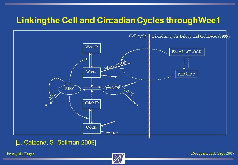Linking the Cell and Circadian Cycles through Wee 1 Cell cycle Circadian cycle Leloup and Goldbeter (1999) Wee 1 P BMAL 1/CLOCK NA Wee 1 . . W . . pre. MPF A m. R ee 1 PC Cdc 25 P Cdc 25 PER/CRY AP C. . . . [L. Calzone, S. Soliman 2006] L François Fages Rocquencourt, Sep. 2007

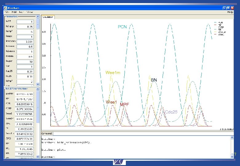PCN Wee 1 m BN Wee 1 MPF Cdc 25 François Fages Rocquencourt, Sep. 2007

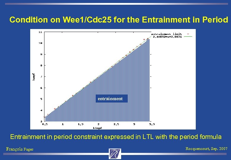Condition on Wee 1/Cdc 25 for the Entrainment in Period entrainment Entrainment in period constraint expressed in LTL with the period formula François Fages Rocquencourt, Sep. 2007

3. 2. Inferring Rules from Temporal Properties Given • a BIOCHAM model (background knowledge) • a set of properties formalized in temporal logic learn • revisions of the reaction model, i. e. rules to delete and rules to add such that the revised model satisfies the properties François Fages Rocquencourt, Sep. 2007

Model Revision from Temporal Properties • Background knowledge T: BIOCHAM model • reaction rule language: complexation, phosphorylation, … • Examples φ: biological properties formalized in temporal logic language • • Reachability Checkpoints Stable states Oscillations • Bias R: Reaction rule patterns or parameter ranges • Kind of rules to add or delete Find a revision T’ of T such that T’ |= φ François Fages Rocquencourt, Sep. 2007

Model Revision Algorithm General idea of constraint programming: replace a generate-and-test algorithm by a constrain-and-generate algorithm. Anticipate whether one has to add or remove a rule. • Positive ECTL formula: if false, remains false after removing a rule • EF(φ) where φ is a boolean formula (pure state description) • Oscil(φ) • Negative ACTL formula: if false, remains false after adding a rule • AG(φ) where φ is a boolean formula, • Checkpoint(a, b): ¬E(¬a. Ub) • Remove a rule on the path given by the model checker (why command) • Unclassified CTL formulae François Fages Rocquencourt, Sep. 2007

Example: Cell Cycle Control Model Tyson 91] [ MA(k 1) for MA(k 2) for MA(K 7) for _ => Cyclin => _. Cyclin~{p 1} => _. MA(k 8) for MA(k 9) for Cdc 2 => Cdc 2~{p 1} =>Cdc 2. MA(k 3) for Cyclin+Cdc 2~{p 1} => Cdc 2~{p 1}-Cyclin~{p 1}. MA(k 4 p) for Cdc 2~{p 1}-Cyclin~{p 1} => Cdc 2 -Cyclin~{p 1}. k 4*[Cdc 2 -Cyclin~{p 1}]^2*[Cdc 2~{p 1}-Cyclin~{p 1}] for Cdc 2~{p 1}-Cyclin~{p 1} =[Cdc 2 -Cyclin~{p 1}] => Cdc 2 -Cyclin~{p 1}. MA(k 5) for Cdc 2 -Cyclin~{p 1} => Cdc 2~{p 1}-Cyclin~{p 1}. MA(k 6) for Cdc 2 -Cyclin~{p 1} => Cdc 2+Cyclin~{p 1}. François Fages Rocquencourt, Sep. 2007

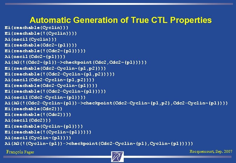Automatic Generation of True CTL Properties Ei(reachable(Cyclin))) Ei(reachable(!(Cyclin)))) Ai(oscil(Cyclin))) Ei(reachable(Cdc 2~{p 1}))) Ei(reachable(!(Cdc 2~{p 1})))) Ai(oscil(Cdc 2~{p 1}))) Ai(AG(!(Cdc 2~{p 1})->checkpoint(Cdc 2, Cdc 2~{p 1})))) Ei(reachable(Cdc 2 -Cyclin~{p 1, p 2}))) Ei(reachable(!(Cdc 2 -Cyclin~{p 1, p 2})))) Ai(oscil(Cdc 2 -Cyclin~{p 1, p 2}))) Ei(reachable(Cdc 2 -Cyclin~{p 1}))) Ei(reachable(!(Cdc 2 -Cyclin~{p 1})))) Ai(oscil(Cdc 2 -Cyclin~{p 1}))) Ai(AG(!(Cdc 2 -Cyclin~{p 1})->checkpoint(Cdc 2 -Cyclin~{p 1, p 2}, Cdc 2 -Cyclin~{p 1}))) Ei(reachable(Cdc 2))) Ei(reachable(!(Cdc 2)))) Ai(oscil(Cdc 2))) Ei(reachable(Cyclin~{p 1}))) Ei(reachable(!(Cyclin~{p 1})))) Ai(oscil(Cyclin~{p 1}))) Ai(AG(!(Cyclin~{p 1})->checkpoint(Cdc 2 -Cyclin~{p 1}, Cyclin~{p 1})))) François Fages Rocquencourt, Sep. 2007

Rule Deletion biocham: delete_rules(Cdc 2 => Cdc 2~{p 1}). biocham: check_all. First formula not satisfied Ei(EF(Cdc 2 -Cyclin~{p 1})) François Fages Rocquencourt, Sep. 2007

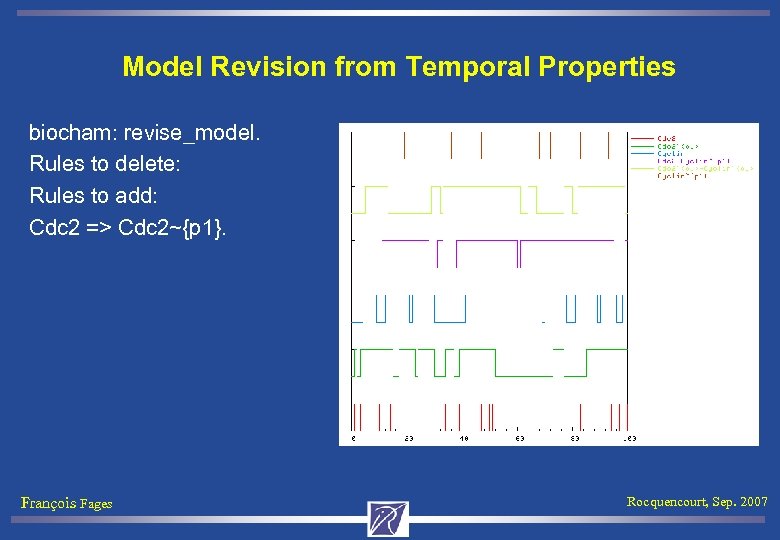Model Revision from Temporal Properties biocham: revise_model. Rules to delete: Rules to add: Cdc 2 => Cdc 2~{p 1}. François Fages Rocquencourt, Sep. 2007

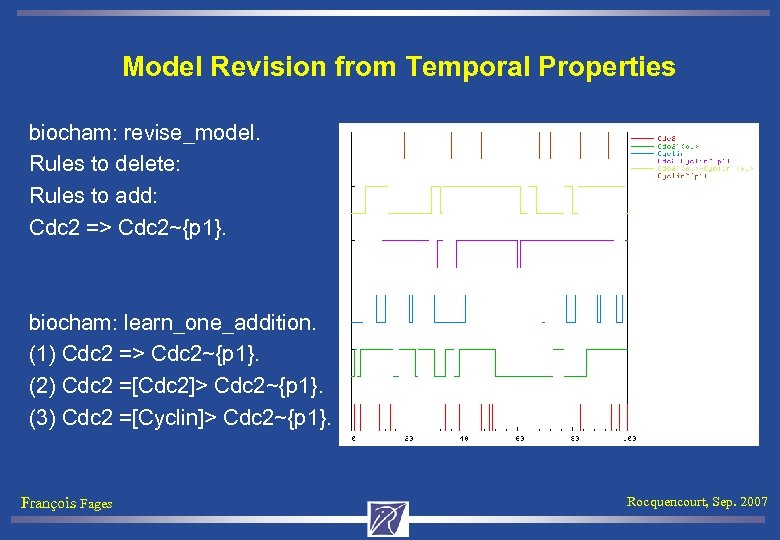Model Revision from Temporal Properties biocham: revise_model. Rules to delete: Rules to add: Cdc 2 => Cdc 2~{p 1}. biocham: learn_one_addition. (1) Cdc 2 => Cdc 2~{p 1}. (2) Cdc 2 =[Cdc 2]> Cdc 2~{p 1}. (3) Cdc 2 =[Cyclin]> Cdc 2~{p 1}. François Fages Rocquencourt, Sep. 2007

Conclusion • Temporal logic with constraints is powerful enough to express both qualitative and quantitative biological properties of systems François Fages Rocquencourt, Sep. 2007

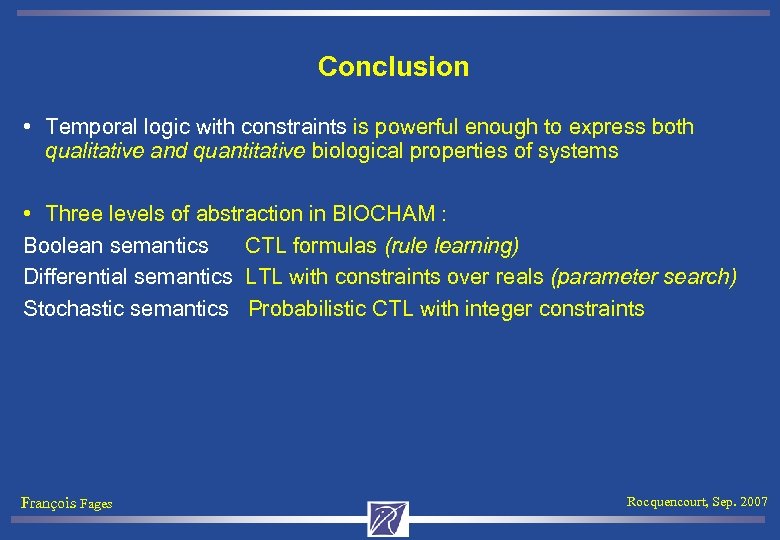Conclusion • Temporal logic with constraints is powerful enough to express both qualitative and quantitative biological properties of systems • Three levels of abstraction in BIOCHAM : Boolean semantics CTL formulas (rule learning) Differential semantics LTL with constraints over reals (parameter search) Stochastic semantics Probabilistic CTL with integer constraints François Fages Rocquencourt, Sep. 2007

Conclusion • Temporal logic with constraints is powerful enough to express both qualitative and quantitative biological properties of systems • Three levels of abstraction in BIOCHAM : Boolean semantics CTL formulas (rule learning) Differential semantics LTL with constraints over reals (parameter search) Stochastic semantics Probabilistic CTL with integer constraints • Parameter search from temporal properties proved useful and complementary to bifurcation theory tools (Xppaut) François Fages Rocquencourt, Sep. 2007

Conclusion • Temporal logic with constraints is powerful enough to express both qualitative and quantitative biological properties of systems • Three levels of abstraction in BIOCHAM : Boolean semantics CTL formulas (rule learning) Differential semantics LTL with constraints over reals (parameter search) Stochastic semantics Probabilistic CTL with integer constraints • Parameter search from temporal properties proved useful and complementary to bifurcation theory tools (Xppaut) • Rule inference from temporal properties still in infancy, to be optimized and improved by types (e. g. protein functions, computed by abstract interpretation) François Fages Rocquencourt, Sep. 2007

Collaborations STREP APr. IL 2 : Luc de Raedt, Univ. Freiburg, Stephen Muggleton, IC , … • Learning in a probabilistic logic setting (finished) ARC MOCA : • modularity, compositionality and abstraction No. E REWERSE : semantic web, François Bry, Münich, Rolf Backofen, • Connecting Biocham to gene and protein ontologies (types) STREP TEMPO : Cancer chronotherapies, INSERM Villejuif, F. Lévi; Bang: J. Clairambault, Contraintes: S. Soliman • Coupled models of cell cycle, circadian cycle, cytotoxic drugs. INRA Tours : E. Reiter, D. Heitzler, Sysiphe : F. Clément • Model of FSH signalling. François Fages Rocquencourt, Sep. 2007