Self-optimizing control Theory 1 Outline Skogestad

Self-optimizing control Theory 1

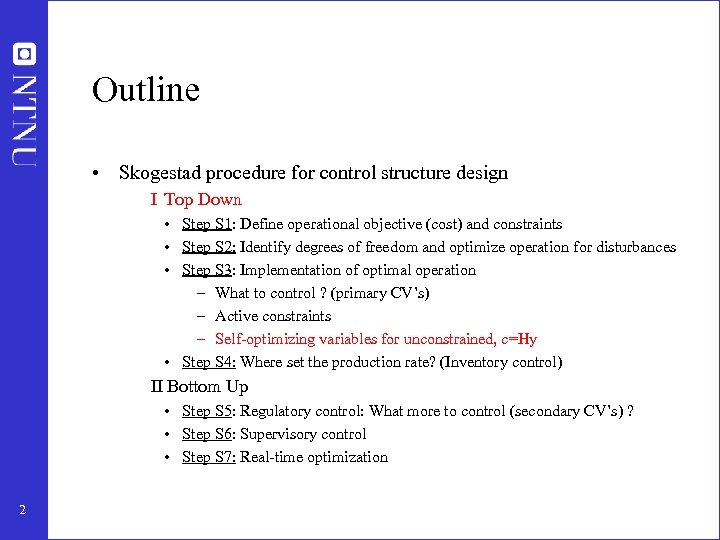Outline • Skogestad procedure for control structure design I Top Down • Step S 1: Define operational objective (cost) and constraints • Step S 2: Identify degrees of freedom and optimize operation for disturbances • Step S 3: Implementation of optimal operation – What to control ? (primary CV’s) – Active constraints – Self-optimizing variables for unconstrained, c=Hy • Step S 4: Where set the production rate? (Inventory control) II Bottom Up • Step S 5: Regulatory control: What more to control (secondary CV’s) ? • Step S 6: Supervisory control • Step S 7: Real-time optimization 2

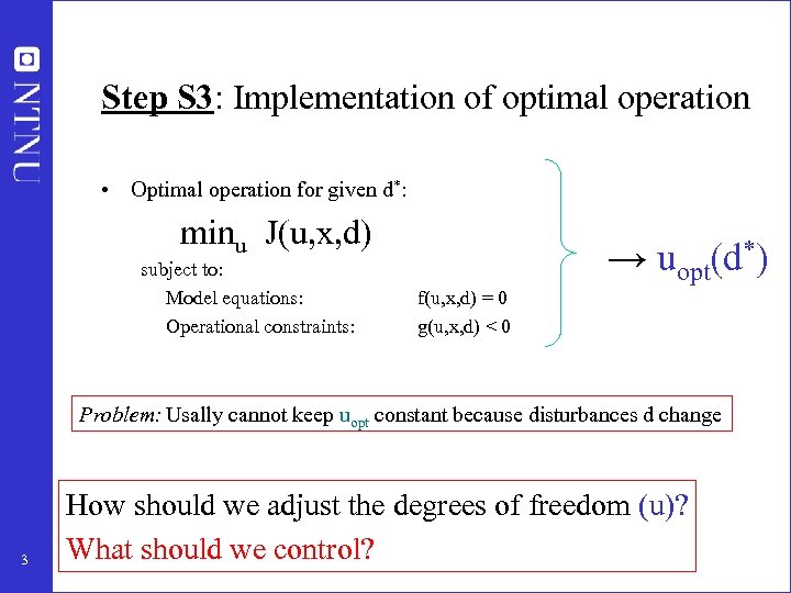Step S 3: Implementation of optimal operation • Optimal operation for given d*: minu J(u, x, d) subject to: Model equations: Operational constraints: → uopt(d*) f(u, x, d) = 0 g(u, x, d) < 0 Problem: Usally cannot keep uopt constant because disturbances d change 3 How should we adjust the degrees of freedom (u)? What should we control?

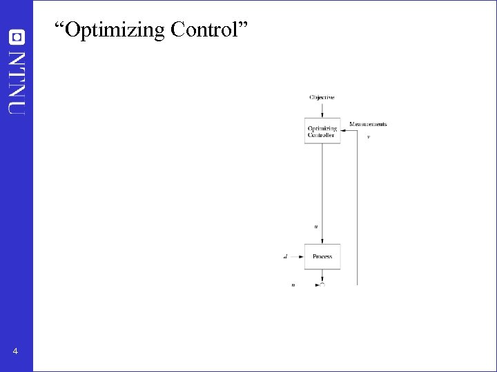“Optimizing Control” y 4

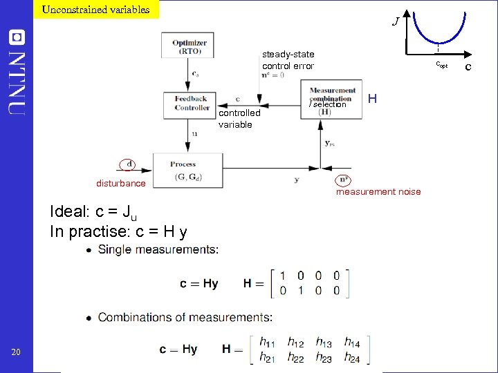
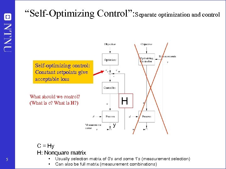“Self-Optimizing Control”: Separate optimization and control Self-optimizing control: Constant setpoints give acceptable loss What should we control? (What is c? What is H? ) H y C = Hy H: Nonquare matrix 5 • • Usually selection matrix of 0’s and some 1’s (measurement selection) Can also be full matrix (measurement combinations)

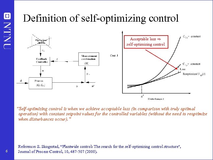Definition of self-optimizing control Acceptable loss ) self-optimizing control “Self-optimizing control is when we achieve acceptable loss (in comparison with truly optimal operation) with constant setpoint values for the controlled variables (without the need to reoptimize when disturbances occur). ” 6 Reference: S. Skogestad, “Plantwide control: The search for the self-optimizing control structure'', Journal of Process Control, 10, 487 -507 (2000).

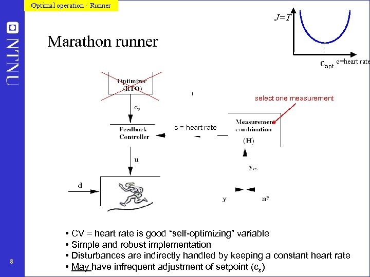Optimal operation - Runner J=T Marathon runner copt c=heart rate select one measurement c = heart rate 8 • CV = heart rate is good “self-optimizing” variable • Simple and robust implementation • Disturbances are indirectly handled by keeping a constant heart rate • May have infrequent adjustment of setpoint (cs)

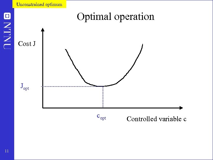Unconstrained optimum Optimal operation Cost J Jopt copt 11 Controlled variable c

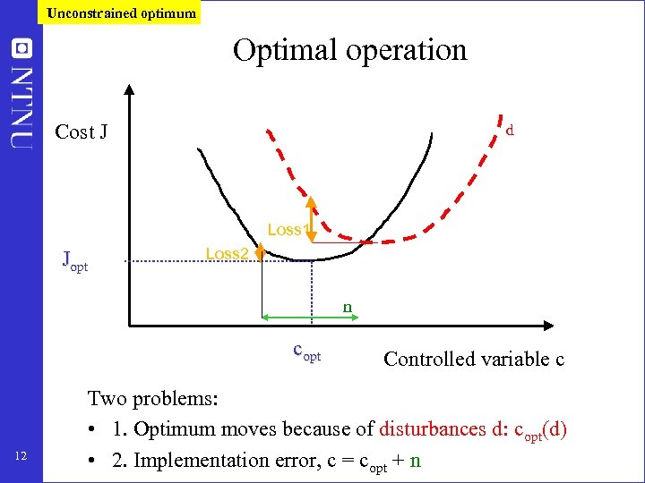Unconstrained optimum Optimal operation Cost J d Loss 1 Jopt Loss 2 n copt 12 Controlled variable c Two problems: • 1. Optimum moves because of disturbances d: copt(d) • 2. Implementation error, c = copt + n

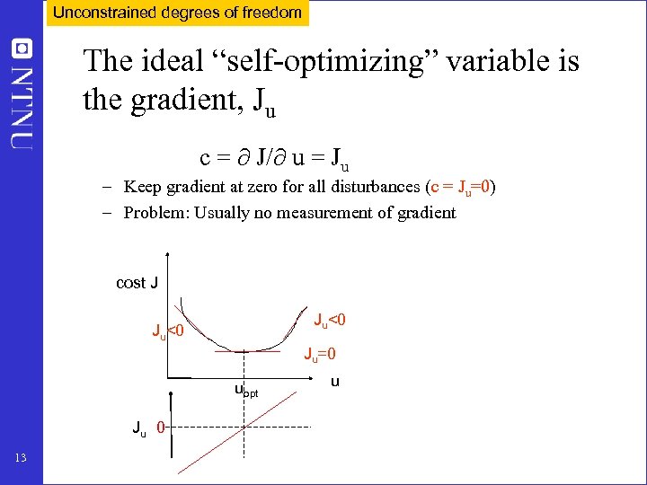Unconstrained degrees of freedom The ideal “self-optimizing” variable is the gradient, Ju c = J/ u = Ju – Keep gradient at zero for all disturbances (c = Ju=0) – Problem: Usually no measurement of gradient cost J Ju<0 Ju=0 uopt Ju 0 13 u

J J>Jmin J Jmin: Forces us to be nonoptimal (two steady states: may require strange operation)

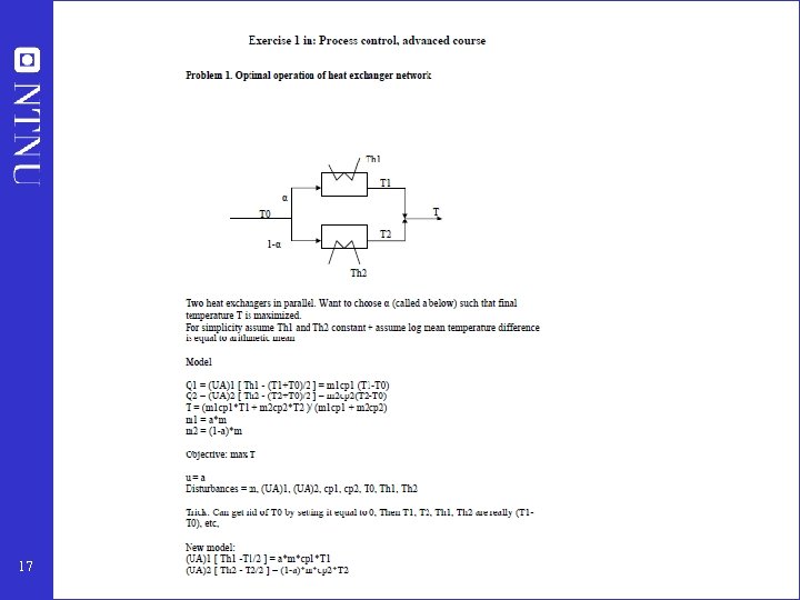
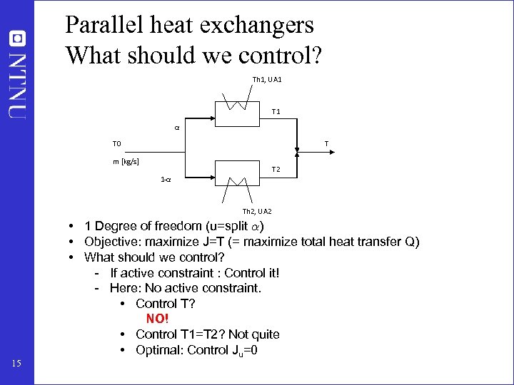Parallel heat exchangers What should we control? Th 1, UA 1 T 1 α T 0 T m [kg/s] T 2 1 -α Th 2, UA 2 15 • 1 Degree of freedom (u=split ®) • Objective: maximize J=T (= maximize total heat transfer Q) • What should we control? - If active constraint : Control it! - Here: No active constraint. • Control T? NO! • Control T 1=T 2? Not quite • Optimal: Control Ju=0

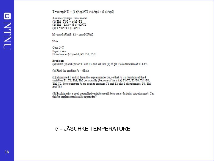
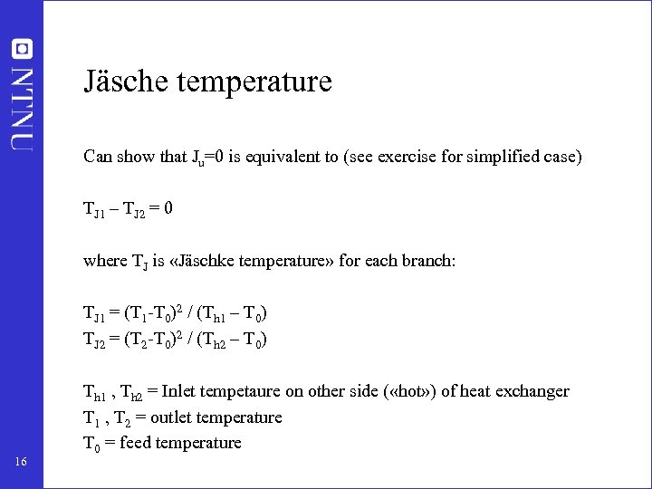Jäsche temperature Can show that Ju=0 is equivalent to (see exercise for simplified case) TJ 1 – TJ 2 = 0 where TJ is «Jäschke temperature» for each branch: TJ 1 = (T 1 -T 0)2 / (Th 1 – T 0) TJ 2 = (T 2 -T 0)2 / (Th 2 – T 0) 16 Th 1 , Th 2 = Inlet tempetaure on other side ( «hot» ) of heat exchanger T 1 , T 2 = outlet temperature T 0 = feed temperature

17

c = JÄSCHKE TEMPERATURE 18

Unconstrained variables J steady-state control error controlled variable disturbance Ideal: c = Ju In practise: c = H y 20 copt / selection H measurement noise c

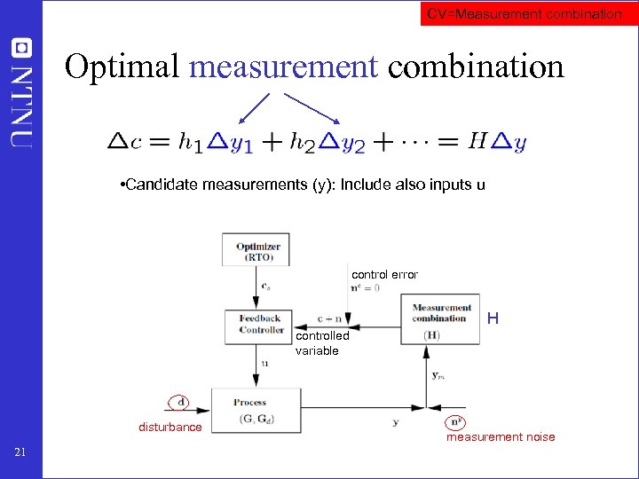CV=Measurement combination Optimal measurement combination • Candidate measurements (y): Include also inputs u control error H controlled variable disturbance 21 measurement noise

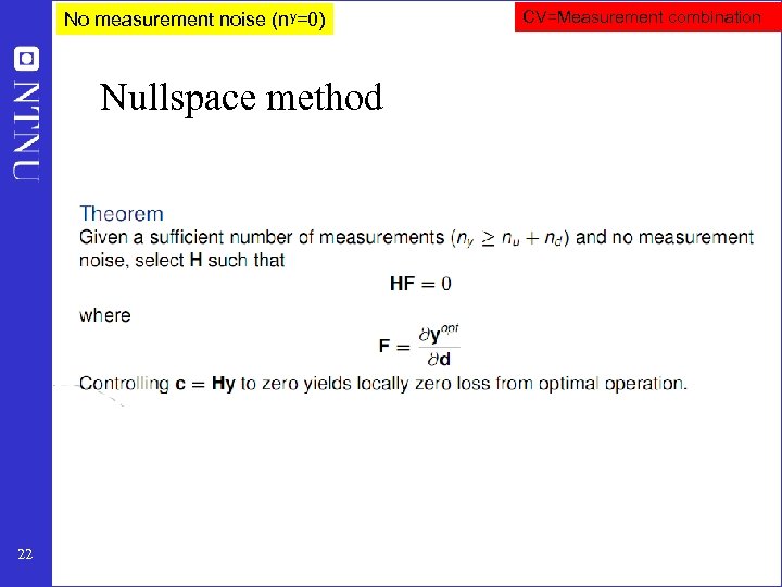No measurement noise (ny=0) Nullspace method 22 CV=Measurement combination

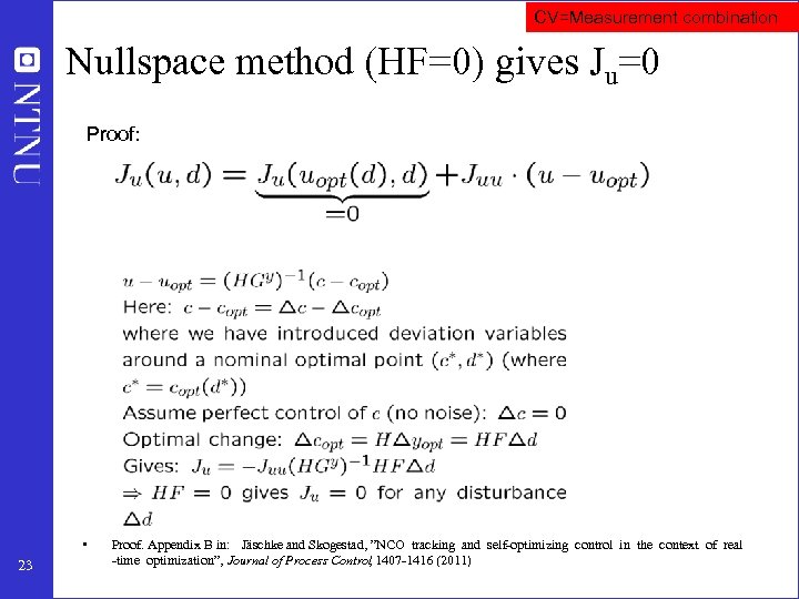CV=Measurement combination Nullspace method (HF=0) gives Ju=0 Proof: • 23 Proof. Appendix B in: Jäschke and Skogestad, ”NCO tracking and self-optimizing control in the context of real -time optimization”, Journal of Process Control 1407 -1416 (2011) ,

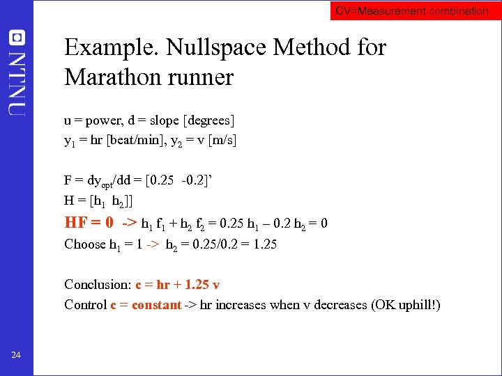CV=Measurement combination Example. Nullspace Method for Marathon runner u = power, d = slope [degrees] y 1 = hr [beat/min], y 2 = v [m/s] F = dyopt/dd = [0. 25 -0. 2]’ H = [h 1 h 2]] HF = 0 -> h 1 f 1 + h 2 f 2 = 0. 25 h 1 – 0. 2 h 2 = 0 Choose h 1 = 1 -> h 2 = 0. 25/0. 2 = 1. 25 Conclusion: c = hr + 1. 25 v Control c = constant -> hr increases when v decreases (OK uphill!) 24

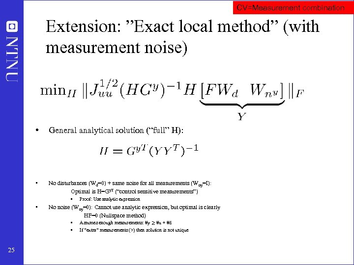CV=Measurement combination Extension: ”Exact local method” (with measurement noise) • General analytical solution (“full” H): • No disturbances (Wd=0) + same noise for all measurements (W ny=I): Optimal is H=Gy. T (“control sensitive measurements”) • • No noise (Wny=0): Cannot use analytic expression, but optimal is clearly HF=0 (Nullspace method) • • 25 Proof: Use analytic expression Assumes enough measurements: #y ¸ #u + #d If “extra” measurements (>) then solution is not unique

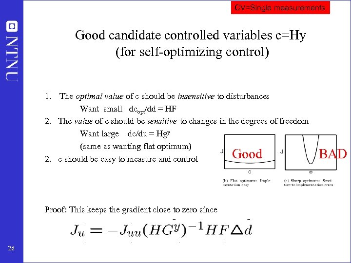CV=Single measurements Good candidate controlled variables c=Hy (for self-optimizing control) 1. The optimal value of c should be insensitive to disturbances Want small dcopt/dd = HF 2. The value of c should be sensitive to changes in the degrees of freedom Want large dc/du = Hgy (same as wanting flat optimum) Good 2. c should be easy to measure and control Proof: This keeps the gradient close to zero since 26 BAD

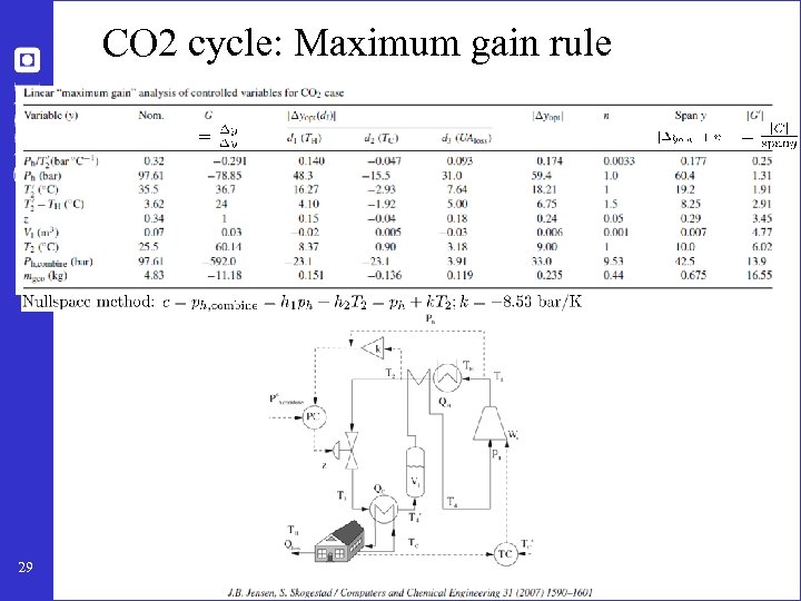
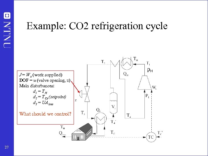Example: CO 2 refrigeration cycle J = W s (work supplied) DOF = u (valve opening, z) Main disturbances: d 1 = T H d 2 = T Cs (setpoint) d 3 = UA loss What should we control? 27 p. H

CO 2 refrigeration cycle Step 1. One (remaining) degree of freedom (u=z) Step 2. Objective function. J = Ws (compressor work) Step 3. Optimize operation for disturbances (d 1=TC, d 2=TH, d 3=UA) • Optimum always unconstrained Step 4. Implementation of optimal operation • No good single measurements (all give large losses): – ph, Th, z, … • Nullspace method: Need to combine nu+nd=1+3=4 measurements to have zero disturbance loss • Simpler: Try combining two measurements. Exact local method: – c = h 1 ph + h 2 Th = ph + k Th; k = -8. 53 bar/K • Nonlinear evaluation of loss: OK! 28

CO 2 cycle: Maximum gain rule 29

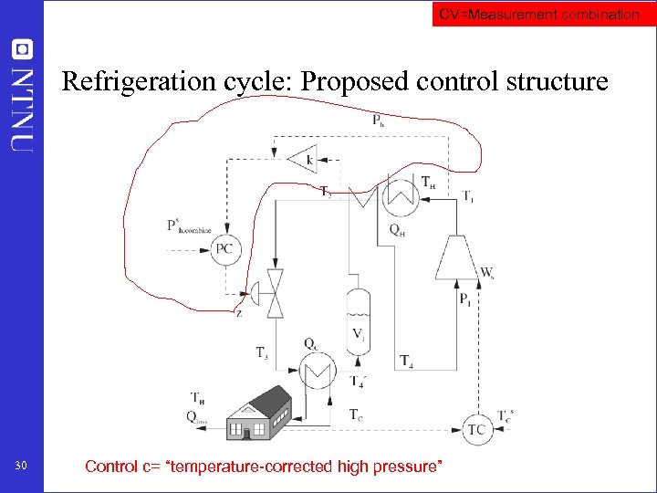CV=Measurement combination Refrigeration cycle: Proposed control structure 30 Control c= “temperature-corrected high pressure”

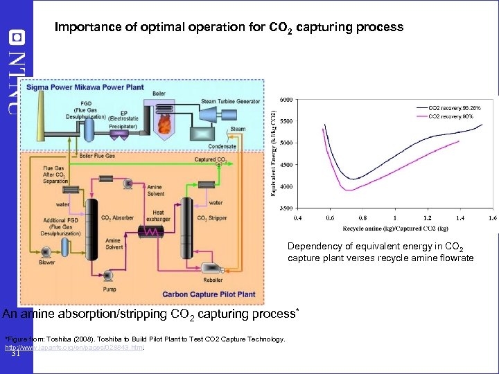Importance of optimal operation for CO 2 capturing process Dependency of equivalent energy in CO 2 capture plant verses recycle amine flowrate An amine absorption/stripping CO 2 capturing process* *Figure from: Toshiba (2008). Toshiba to Build Pilot Plant to Test CO 2 Capture Technology. http: //www. japanfs. org/en/pages/028843. html. 31

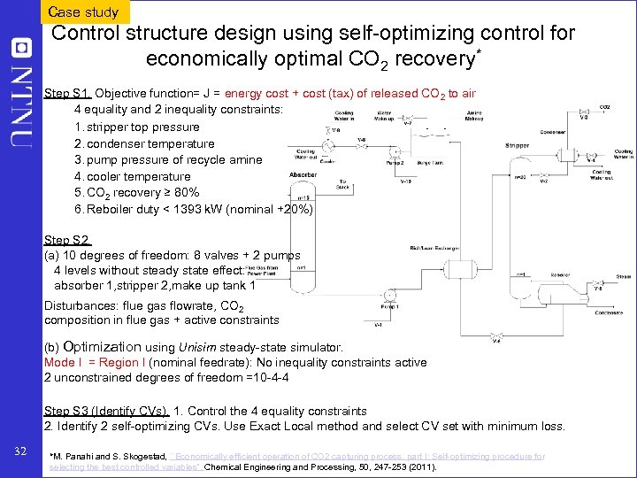Case study Control structure design using self-optimizing control for economically optimal CO 2 recovery* Step S 1. Objective function= J = energy cost + cost (tax) of released CO 2 to air 4 equality and 2 inequality constraints: 1. stripper top pressure 2. condenser temperature 3. pump pressure of recycle amine 4. cooler temperature 5. CO 2 recovery ≥ 80% 6. Reboiler duty < 1393 k. W (nominal +20%) Step S 2. (a) 10 degrees of freedom: 8 valves + 2 pumps 4 levels without steady state effect: absorber 1, stripper 2, make up tank 1 Disturbances: flue gas flowrate, CO 2 composition in flue gas + active constraints (b) Optimization using Unisim steady-state simulator. Mode I = Region I (nominal feedrate): No inequality constraints active 2 unconstrained degrees of freedom =10 -4 -4 Step S 3 (Identify CVs). 1. Control the 4 equality constraints 2. Identify 2 self-optimizing CVs. Use Exact Local method and select CV set with minimum loss. 32 *M. Panahi and S. Skogestad, ``Economically efficient operation of CO 2 capturing process, part I: Self-optimizing procedure for selecting the best controlled variables'', Chemical Engineering and Processing, 50, 247 -253 (2011).

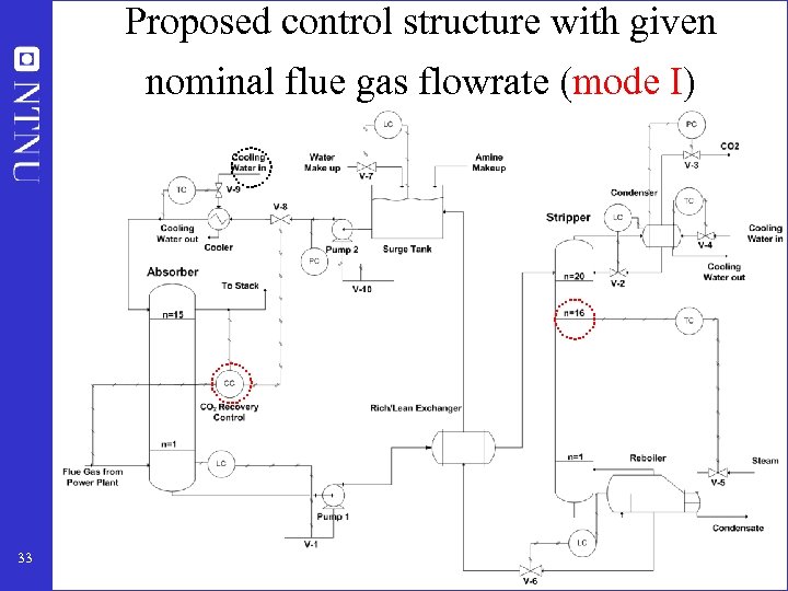Proposed control structure with given nominal flue gas flowrate (mode I) 33

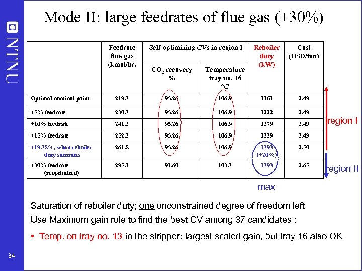Mode II: large feedrates of flue gas (+30%) Feedrate flue gas (kmol/hr) Self-optimizing CVs in region I CO 2 recovery % Temperature tray no. 16 °C Reboiler duty (k. W) Cost (USD/ton) Optimal nominal point 219. 3 95. 26 106. 9 1161 2. 49 +5% feedrate 230. 3 95. 26 106. 9 1222 2. 49 +10% feedrate 241. 2 95. 26 106. 9 1279 2. 49 +15% feedrate 252. 2 95. 26 106. 9 1339 2. 49 +19. 38%, when reboiler duty saturates 261. 8 95. 26 106. 9 1393 (+20%) 2. 50 +30% feedrate (reoptimized) 285. 1 91. 60 103. 3 1393 2. 65 region II max Saturation of reboiler duty; one unconstrained degree of freedom left Use Maximum gain rule to find the best CV among 37 candidates : • Temp. on tray no. 13 in the stripper: largest scaled gain, but tray 16 also OK 34

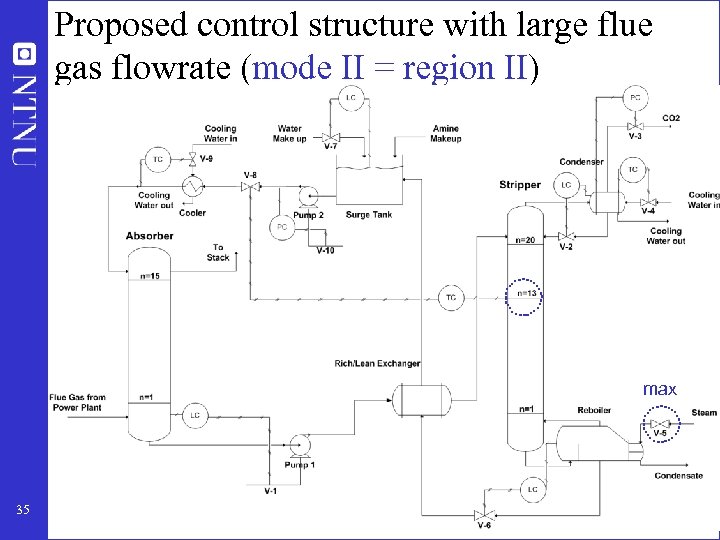Proposed control structure with large flue gas flowrate (mode II = region II) max 35

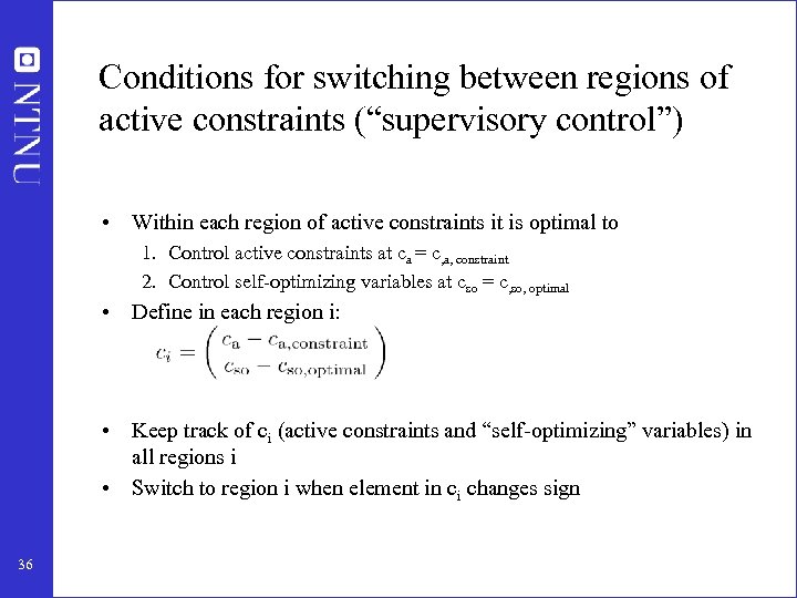Conditions for switching between regions of active constraints (“supervisory control”) • Within each region of active constraints it is optimal to 1. Control active constraints at ca = c, a, constraint 2. Control self-optimizing variables at cso = c, so, optimal • Define in each region i: • Keep track of ci (active constraints and “self-optimizing” variables) in all regions i • Switch to region i when element in ci changes sign 36

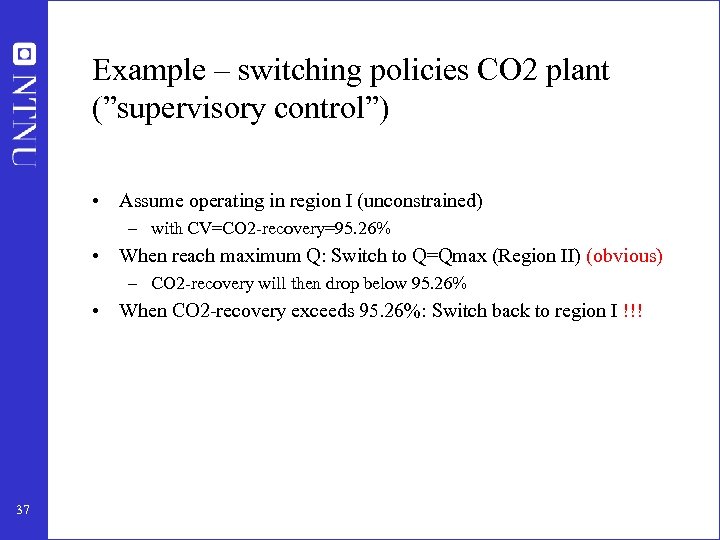Example – switching policies CO 2 plant (”supervisory control”) • Assume operating in region I (unconstrained) – with CV=CO 2 -recovery=95. 26% • When reach maximum Q: Switch to Q=Qmax (Region II) (obvious) – CO 2 -recovery will then drop below 95. 26% • When CO 2 -recovery exceeds 95. 26%: Switch back to region I !!! 37

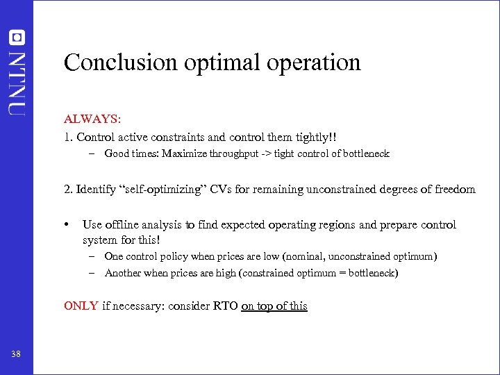Conclusion optimal operation ALWAYS: 1. Control active constraints and control them tightly!! – Good times: Maximize throughput -> tight control of bottleneck 2. Identify “self-optimizing” CVs for remaining unconstrained degrees of freedom • Use offline analysis to find expected operating regions and prepare control system for this! – One control policy when prices are low (nominal, unconstrained optimum) – Another when prices are high (constrained optimum = bottleneck) ONLY if necessary: consider RTO on top of this 38

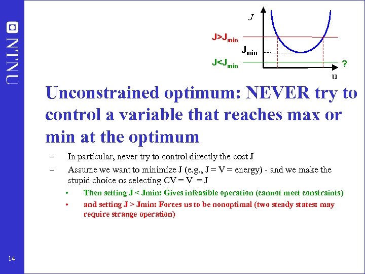
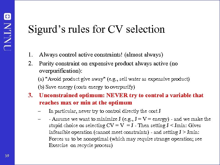Sigurd’s rules for CV selection 1. 2. Always control active constraints! (almost always) Purity constraint on expensive product always active (no overpurification): (a) "Avoid product give away" (e. g. , sell water as expensive product) (b) Save energy (costs energy to overpurify) 3. Unconstrained optimum: NEVER try to control a variable that reaches max or min at the optimum – – 39 In particular, never try to control directly the cost J - Assume we want to minimize J (e. g. , J = V = energy) - and we make the stupid choice os selecting CV = J - Then setting J < Jmin: Gives infeasible operation (cannot meet constraints) - and setting J > Jmin: Forces us to be nonoptimal (which may require strange operation; see Exercise on recycle process)