Selection of Differential Expression Genes in Microarray Experiments

Selection of Differential Expression Genes in Microarray Experiments James J. Chen, Ph. D. Division of Biometry and Risk Assessment National Center for Toxicological Research Food and Drug Administration e-mail: Jchen@nctr. fda. gov FDA/Industry Workshop September 19, 2003

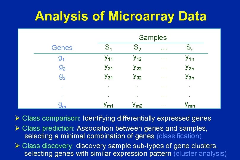Analysis of Microarray Data Genes g 1 g 2 g 3. . gm S 1 y 11 y 21 y 31. . ym 1 Samples S 2 … y 12 … y 22 … y 32 …. …. … ym 2. . . Sn y 1 n y 2 n y 3 n. . ymn Ø Class comparison: Identifying differentially expressed genes Ø Class prediction: Association between genes and samples, selecting a minimal combination of genes (classification). Ø Class discovery: discovery sample sub-types of gene clusters, selecting genes with similar expression pattern (cluster analysis)

Identifying Differentially Expressed Genes An important goal in the data analysis is to identify a set of genes that are differentially expressed among control and treated samples (groups). Ø To identify disease-related, drug-response, or biomarker genes (class comparison). Ø To enhance relationships among genes and samples for clustering or prediction (class prediction or class discovery).

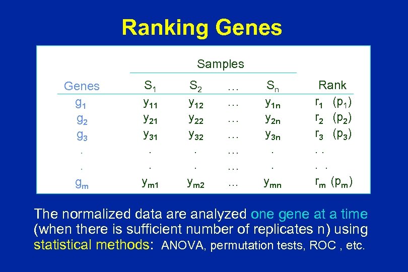Ranking Genes Samples Genes g 1 g 2 g 3. . gm S 1 y 11 y 21 y 31. . ym 1 S 2 y 12 y 22 y 32. . ym 2 … … …. . . Sn y 1 n y 2 n y 3 n. . ymn Rank r 1 (p 1) r 2 (p 2) r 3 (p 3). . rm (pm) The normalized data are analyzed one gene at a time (when there is sufficient number of replicates n) using statistical methods: ANOVA, permutation tests, ROC , etc.

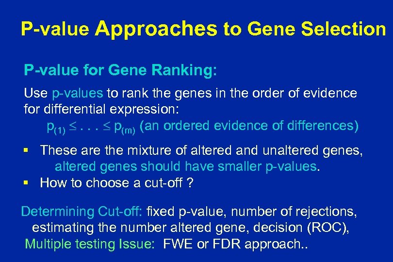P-value Approaches to Gene Selection P-value for Gene Ranking: Use p-values to rank the genes in the order of evidence for differential expression: p(1) . . . p(m) (an ordered evidence of differences) § These are the mixture of altered and unaltered genes, altered genes should have smaller p-values. § How to choose a cut-off ? Determining Cut-off: fixed p-value, number of rejections, estimating the number altered gene, decision (ROC), Multiple testing Issue: FWE or FDR approach. .

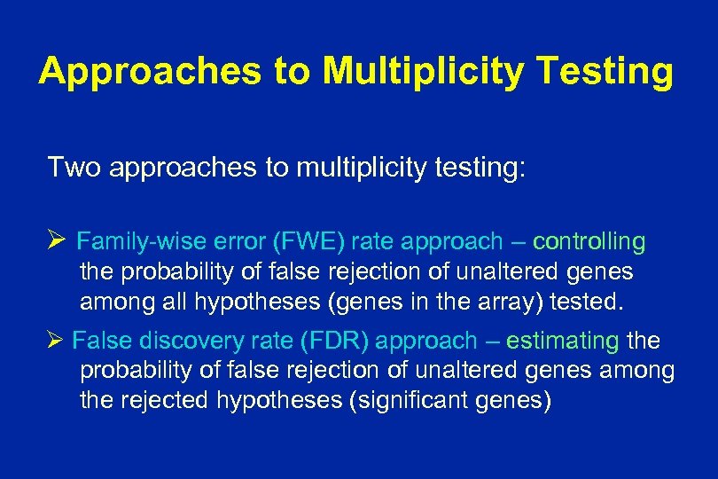Approaches to Multiplicity Testing Two approaches to multiplicity testing: Ø Family-wise error (FWE) rate approach – controlling the probability of false rejection of unaltered genes among all hypotheses (genes in the array) tested. Ø False discovery rate (FDR) approach – estimating the probability of false rejection of unaltered genes among the rejected hypotheses (significant genes)

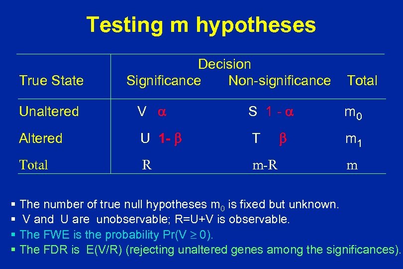Testing m hypotheses True State Decision Significance Non-significance Unaltered V S 1 - Altered U 1 - T Total R m-R Total m 0 m 1 m § The number of true null hypotheses m 0 is fixed but unknown. § V and U are unobservable; R=U+V is observable. § The FWE is the probability Pr(V 0). § The FDR is E(V/R) (rejecting unaltered genes among the significances).

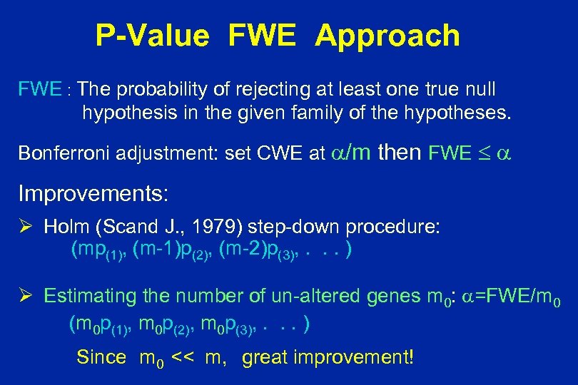P-Value FWE Approach FWE : The probability of rejecting at least one true null hypothesis in the given family of the hypotheses. Bonferroni adjustment: set CWE at /m then FWE Improvements: Ø Holm (Scand J. , 1979) step-down procedure: (mp(1), (m-1)p(2), (m-2)p(3), . . . ) Ø Estimating the number of un-altered genes m 0: =FWE/m 0 (m 0 p(1), m 0 p(2), m 0 p(3), . . . ) Since m 0 << m, great improvement!

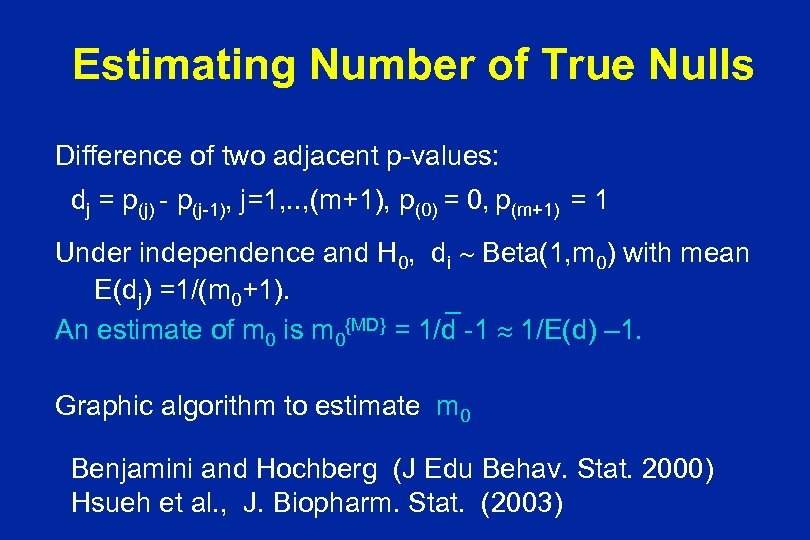Estimating Number of True Nulls Difference of two adjacent p-values: dj = p(j) - p(j-1), j=1, . . , (m+1), p(0) = 0, p(m+1) = 1 Under independence and H 0, di Beta(1, m 0) with mean E(dj) =1/(m 0+1). _ An estimate of m 0 is m 0{MD} = 1/d -1 1/E(d) – 1. Graphic algorithm to estimate m 0 Benjamini and Hochberg (J Edu Behav. Stat. 2000) Hsueh et al. , J. Biopharm. Stat. (2003)

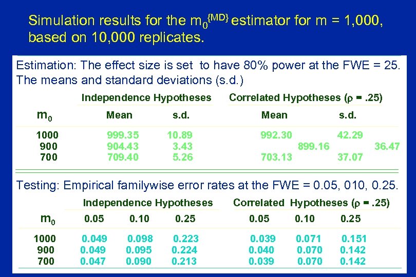Simulation results for the m 0{MD} estimator for m = 1, 000, based on 10, 000 replicates. Estimation: The effect size is set to have 80% power at the FWE = 25. The means and standard deviations (s. d. ) Independence Hypotheses m 0 Mean 1000 900 700 999. 35 904. 43 709. 40 Correlated Hypotheses ( =. 25) s. d. Mean s. d. 10. 89 3. 43 5. 26 992. 30 42. 29 703. 13 899. 16 37. 07 36. 47 Testing: Empirical familywise error rates at the FWE = 0. 05, 010, 0. 25. Independence Hypotheses m 0 1000 900 700 Correlated Hypotheses ( =. 25) 0. 05 0. 10 0. 25 0. 049 0. 047 0. 098 0. 095 0. 090 0. 223 0. 224 0. 213 0. 039 0. 040 0. 039 0. 071 0. 070 0. 151 0. 142

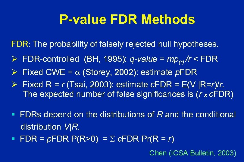P-value FDR Methods FDR: The probability of falsely rejected null hypotheses. Ø FDR-controlled (BH, 1995): q-value = mp(r) /r < FDR Ø Fixed CWE = (Storey, 2002): estimate p. FDR Ø Fixed R = r (Tsai, 2003): estimate c. FDR = E(V |R=r)/r. The expected number of false significances is (r x c. FDR) § FDRs depend on the distributions of R and the conditional distribution V|R. § FDR = p. FDR P(R>0) = c. FDR Pr(R = r) Chen (ICSA Bulletin, 2003)

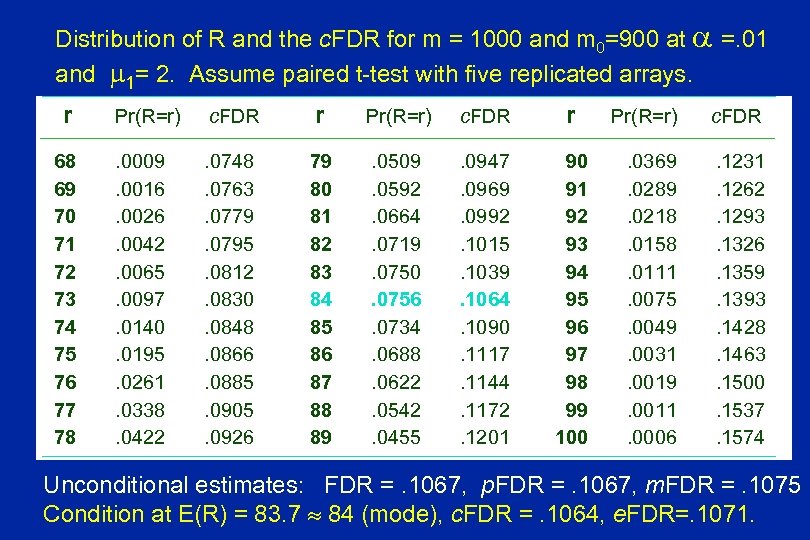Distribution of R and the c. FDR for m = 1000 and m 0=900 at =. 01 and 1= 2. Assume paired t-test with five replicated arrays. r 68 69 70 71 72 73 74 75 76 77 78 Pr(R=r) c. FDR r . 0009. 0016. 0026. 0042. 0065. 0097. 0140. 0195. 0261. 0338. 0422 . 0748. 0763. 0779. 0795. 0812. 0830. 0848. 0866. 0885. 0905. 0926 79 80 81 82 83 84 85 86 87 88 89 . 0509. 0592. 0664. 0719. 0750. 0756. 0734. 0688. 0622. 0542. 0455 . 0947. 0969. 0992. 1015. 1039. 1064. 1090. 1117. 1144. 1172. 1201 90 91 92 93 94 95 96 97 98 99 100 Pr(R=r) c. FDR . 0369. 0289. 0218. 0158. 0111. 0075. 0049. 0031. 0019. 0011. 0006 . 1231. 1262. 1293. 1326. 1359. 1393. 1428. 1463. 1500. 1537. 1574 Unconditional estimates: FDR =. 1067, p. FDR =. 1067, m. FDR =. 1075 Condition at E(R) = 83. 7 84 (mode), c. FDR =. 1064, e. FDR=. 1071.

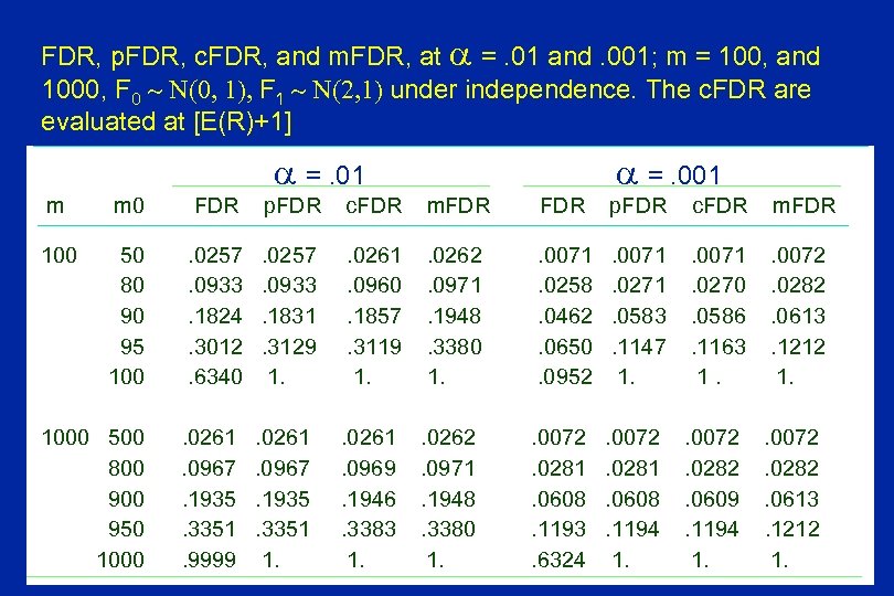FDR, p. FDR, c. FDR, and m. FDR, at =. 01 and. 001; m = 100, and 1000, F 0 N(0, 1), F 1 N(2, 1) under independence. The c. FDR are evaluated at [E(R)+1] =. 01 =. 001 m m 0 FDR p. FDR c. FDR m. FDR 100 50 80 90 95 100 . 0257. 0933. 1824. 3012. 6340 . 0257. 0933. 1831. 3129 1. . 0261. 0960. 1857. 3119 1. . 0262. 0971. 1948. 3380 1. . 0071. 0258. 0462. 0650. 0952 . 0071. 0271. 0583. 1147 1. . 0071. 0270. 0586. 1163 1. . 0072. 0282. 0613. 1212 1. 1000 500 800 950 1000 . 0261. 0967. 1935. 3351. 9999 . 0261. 0967. 1935. 3351 1. . 0261. 0969. 1946. 3383 1. . 0262. 0971. 1948. 3380 1. . 0072. 0281. 0608. 1193. 6324 . 0072. 0281. 0608. 1194 1. . 0072. 0282. 0609. 1194 1. . 0072. 0282. 0613. 1212 1.

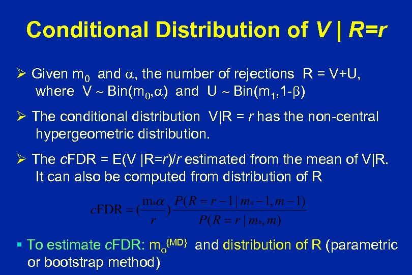Conditional Distribution of V | R=r Ø Given m 0 and , the number of rejections R = V+U, where V Bin(m 0, ) and U Bin(m 1, 1 - ) Ø The conditional distribution V|R = r has the non-central hypergeometric distribution. Ø The c. FDR = E(V |R=r)/r estimated from the mean of V|R. It can also be computed from distribution of R § To estimate c. FDR: mo{MD} and distribution of R (parametric or bootstrap method)

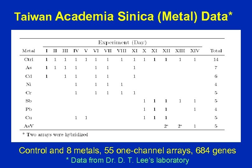Taiwan Academia Sinica (Metal) Data* Control and 8 metals, 55 one-channel arrays, 684 genes * Data from Dr. D. T. Lee’s laboratory

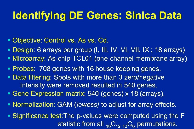Identifying DE Genes: Sinica Data § Objective: Control vs. As vs. Cd. § Design: 6 arrays per group (I, III, IV, VII, IX ; 18 arrays) § Microarray: As-chip-TCL 01 (one-channel membrane array) § Probes: 708 genes with 16 house keeping genes. § Data filtering: Spots with more than 3 zero/negative intensity were removed resulted in 540 genes. § Gene Expression matrix: 540 (genes) x 18 (arrays). § Normalization: GAM (lowess) to adjust for array effects. § Significance test: The p-values were computed using the F statistic from all 18 C 12 12 C 6 permutations.

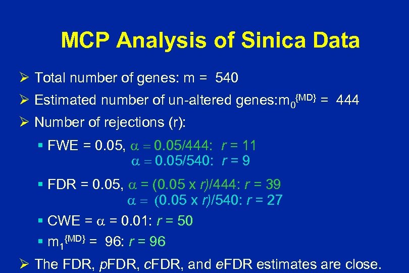MCP Analysis of Sinica Data Ø Total number of genes: m = 540 Ø Estimated number of un-altered genes: m 0{MD} = 444 Ø Number of rejections (r): § FWE = 0. 05, = 0. 05/444: r = 11 = 0. 05/540: r = 9 § FDR = 0. 05, = (0. 05 x r)/444: r = 39 = (0. 05 x r)/540: r = 27 § CWE = = 0. 01: r = 50 § m 1{MD} = 96: r = 96 Ø The FDR, p. FDR, c. FDR, and e. FDR estimates are close.

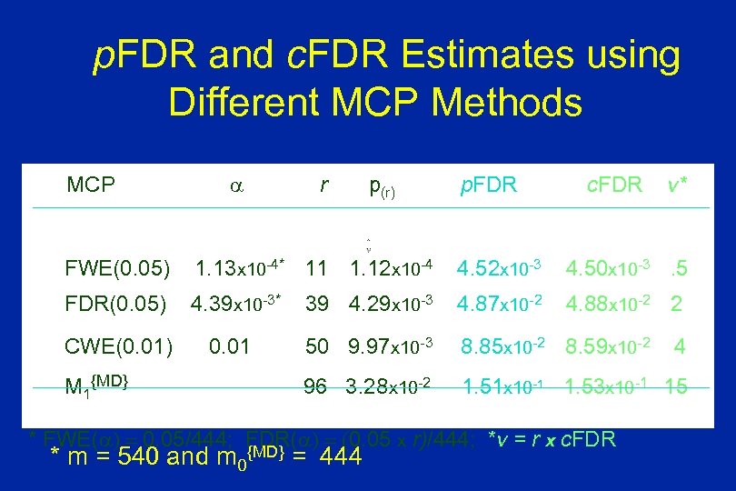p. FDR and c. FDR Estimates using Different MCP Methods MCP r p(r) p. FDR c. FDR v* FWE(0. 05) 1. 13 x 10 -4* 11 1. 12 x 10 -4 4. 52 x 10 -3 4. 50 x 10 -3. 5 FDR(0. 05) 4. 39 x 10 -3* 39 4. 29 x 10 -3 4. 87 x 10 -2 4. 88 x 10 -2 2 CWE(0. 01) 0. 01 50 9. 97 x 10 -3 8. 85 x 10 -2 8. 59 x 10 -2 96 3. 28 x 10 -2 1. 51 x 10 -1 1. 53 x 10 -1 15 M 1{MD} * FWE( ) = 0. 05/444; FDR( ) = (0. 05 x r)/444; *v = r x c. FDR {MD} * m = 540 and m 0 = 444 4

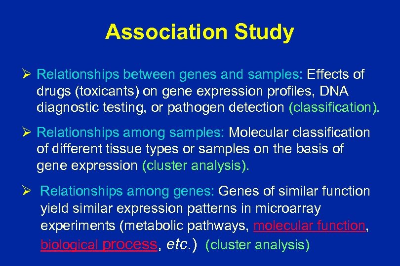Association Study Ø Relationships between genes and samples: Effects of drugs (toxicants) on gene expression profiles, DNA diagnostic testing, or pathogen detection (classification). Ø Relationships among samples: Molecular classification of different tissue types or samples on the basis of gene expression (cluster analysis). Ø Relationships among genes: Genes of similar function yield similar expression patterns in microarray experiments (metabolic pathways, molecular function, biological process, etc. ) (cluster analysis)

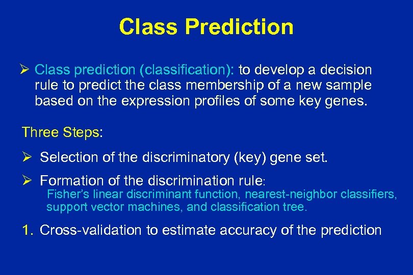Class Prediction Ø Class prediction (classification): to develop a decision rule to predict the class membership of a new sample based on the expression profiles of some key genes. Three Steps: Ø Selection of the discriminatory (key) gene set. Ø Formation of the discrimination rule: Fisher’s linear discriminant function, nearest-neighbor classifiers, support vector machines, and classification tree. 1. Cross-validation to estimate accuracy of the prediction

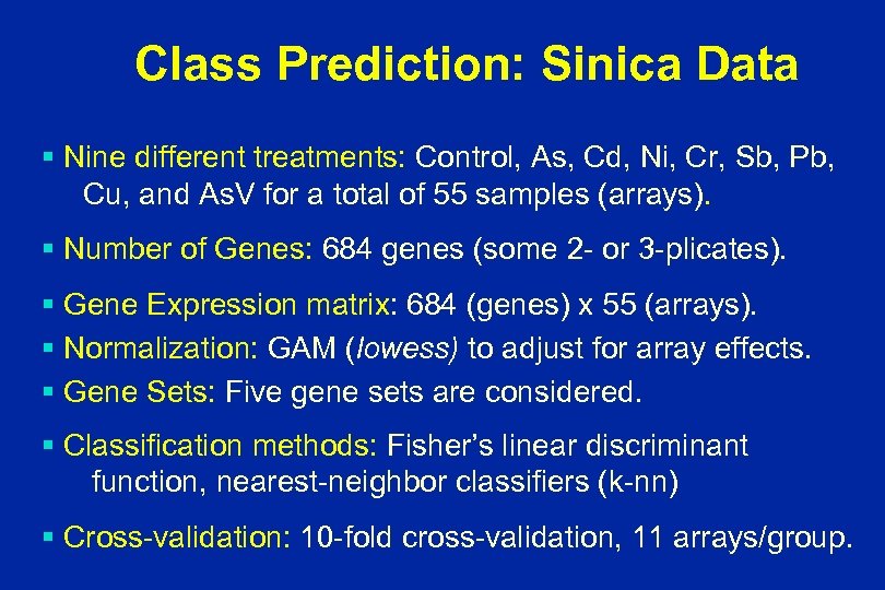Class Prediction: Sinica Data § Nine different treatments: Control, As, Cd, Ni, Cr, Sb, Pb, Cu, and As. V for a total of 55 samples (arrays). § Number of Genes: 684 genes (some 2 - or 3 -plicates). § Gene Expression matrix: 684 (genes) x 55 (arrays). § Normalization: GAM (lowess) to adjust for array effects. § Gene Sets: Five gene sets are considered. § Classification methods: Fisher’s linear discriminant function, nearest-neighbor classifiers (k-nn) § Cross-validation: 10 -fold cross-validation, 11 arrays/group.

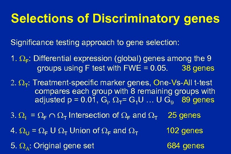Selections of Discriminatory genes Significance testing approach to gene selection: 1. WF: Differential expression (global) genes among the 9 groups using F test with FWE = 0. 05. 38 genes 2. WT: Treatment-specific marker genes, One-Vs-All t-test compares each group with 8 remaining groups with adjusted p = 0. 01, Gi. WT= G 1 U … U G 9 89 genes 3. WI = WF WT Intersection of WF and WT 25 genes 4. WU = WF U WT Union of WF and WT 102 genes 5. WA: Original gene set 684 genes

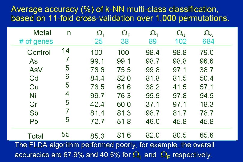Average accuracy (%) of k-NN multi-classification, based on 11 -fold cross-validation over 1, 000 permutations. Metal # of genes Control As As. V Cd Cu Ni Cr Sb Pb n WI 25 WF 38 WT 89 WU 102 WA 684 14 7 5 6 5 4 5 7 5 100 99. 1 78. 6 84. 4 78. 5 99. 7 42. 4 81. 4 72. 7 100 99. 1 75. 5 82. 0 61. 6 76. 3 60. 0 81. 3 51. 8 98. 4 98. 7 99. 8 81. 8 38. 2 99. 5 37. 1 98. 7 46. 0 98. 8 97. 1 81. 5 41. 5 97. 8 97. 1 81. 7 45. 8 79. 0 96. 6 38. 7 50. 4 57. 1 94. 9 18. 3 78. 7 45. 8 55 81. 6 82. 0 80. 5 65. 6 Total 85. 3 The FLDA algorithm performed poorly, for example, the overall accuracies are 67. 9% and 40. 5% for WI and WF respectively.

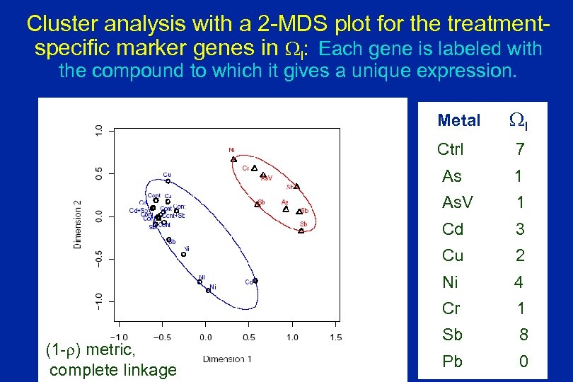Cluster analysis with a 2 -MDS plot for the treatmentspecific marker genes in WI: Each gene is labeled with the compound to which it gives a unique expression. Metal WI Ctrl As 1 As. V 1 Cd 3 Cu 2 Ni 4 Cr (1 -r) metric, complete linkage 7 1 Sb 8 Pb 0

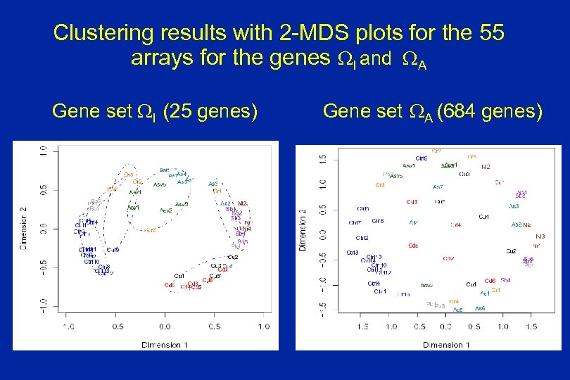Clustering results with 2 -MDS plots for the 55 arrays for the genes WI and WA Gene set WI (25 genes) Gene set WA (684 genes)

Acknowledgements Collaborators and Contributors § Dr. Frank Sistare & Staff § Dr. Sue-Jane Wang § Dr. T-C Lee & Staff § Dr. C-h Chen & Staff (CDER/FDA; Merck) (CDER/FDA) (Academia Sinica, Taiwan) § Dr. Suzanne Morris & Staff § Dr. Jim Fuscoe & Staff § Dr. Ralph Kodell § Dr. Robert Delongchamp (NCTR) (NCTR) § Dr. Hueymiin Hsueh § Dr. Chen-an Tsai § Ms. Yi-Ju Chen (Cheng-chi Univ. , Taiwan) (NCTR) (Pen State, NCTR)