Marfurt K. 1 - Introduction.ppt
- Количество слайдов: 48

Seismic Attribute Mapping of Structure and Stratigraphy Kurt J. Marfurt (AGL, University of Houston)

Seismic Attribute Mapping of Structure and Stratigraphy Sponsored by
Attributes: Capturing an interpreter’s thoughts with a computer algorithm The “Big Book” Chopra and Marfurt Satinder Chopra, ARCIS to appear “late 2006” to be published by SEG www. nationalgeographic. org
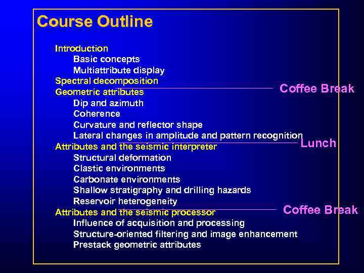
Course Outline Introduction Basic concepts Multiattribute display Spectral decomposition Coffee Break Geometric attributes Dip and azimuth Coherence Curvature and reflector shape Lateral changes in amplitude and pattern recognition Lunch Attributes and the seismic interpreter Structural deformation Clastic environments Carbonate environments Shallow stratigraphy and drilling hazards Reservoir heterogeneity Coffee Break Attributes and the seismic processor Influence of acquisition and processing Structure-oriented filtering and image enhancement Prestack geometric attributes
Apologies and Acknowledgements Many of the examples have come from the published literature: • There are more folks than Marfurt and Chopra working on attributes! We want to show that even though it took more effort to clear the figures. • Thanks to those who provided us with figures! • Most geoscientists are now interpreters rather than researchers and processors – We’ve therefore replaced the math with equivalent figures, cartoons, and examples. • The publications on the CD contain details and equations. • The examples are limited by our work experience. Let us know if you have an excellent example you would like to see published and share!
1 a: Basic Concepts After this section you should be able to: • put attributes in their historical perspective • visualize the Hilbert transform of the data by looking at the original seismic trace • use complex trace attributes as building blocks for interpretation • relate definitions of attributes used in this class to those you use in your work environment
Definition of Seismic Attributes Seismic attributes are specific measures of geometric, kinematic, dynamic, or statistical features derived from seismic data. ‘General’ attributes include: • Reflector amplitude, • Reflector time • Reflector dip and azimuth • Complex amplitude and frequency • Illumination • Edge detection/coherence • AVO • Spectral decomposition These have a physical as well as a statistical basis! There are hundreds of sometimes statistically valid ‘specific’ attributes! (Liner et al. , 2004)
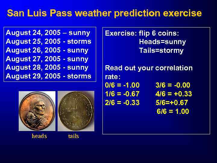
San Luis Pass weather prediction exercise August 24, 2005 – sunny August 25, 2005 - storms August 26, 2005 - sunny August 27, 2005 - sunny August 28, 2005 - sunny August 29, 2005 - storms heads tails Exercise: flip 6 coins: Heads=sunny Tails=stormy Read out your correlation rate: 0/6 = -1. 00 3/6 = -0. 00 1/6 = -0. 67 4/6 = +0. 33 2/6 = -0. 33 5/6=+0. 67 6/6 = 1. 00

San Luis Pass weather prediction exercise Which coins best predict the weather in San Luis Pass? Should Marfurt go fishing based on • Dollars? • Pesos? • Euros? • Won? • Rials? • …
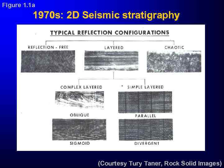
Figure 1. 1 a 1970 s: 2 D Seismic stratigraphy (Courtesy Tury Taner, Rock Solid Images)
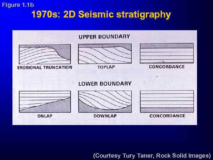
Figure 1. 1 b 1970 s: 2 D Seismic stratigraphy (Courtesy Tury Taner, Rock Solid Images)
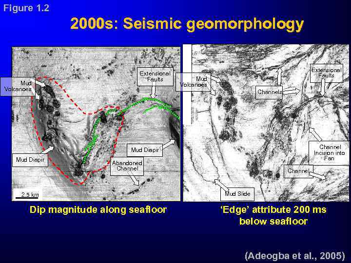
Figure 1. 2 2000 s: Seismic geomorphology Mud Volcanoes Extensional Faults Mud Volcanoes Channel Incision into Fan Mud Diapir Abandoned Channel 2. 5 km Dip magnitude along seafloor Channel Mud Slide ‘Edge’ attribute 200 ms below seafloor (Adeogba et al. , 2005)
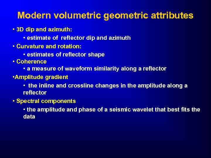
Modern volumetric geometric attributes • 3 D dip and azimuth: • estimate of reflector dip and azimuth • Curvature and rotation: • estimates of reflector shape • Coherence • a measure of waveform similarity along a reflector • Amplitude gradient • the inline and crossline changes in the amplitude along a reflector • Spectral components • the amplitude and phase of a seismic wavelet that best fits the data
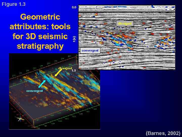
Figure 1. 3 0. 0 divergent t (s) Geometric attributes: tools for 3 D seismic stratigraphy convergent divergent 1. 5 convergent (Barnes, 2002)
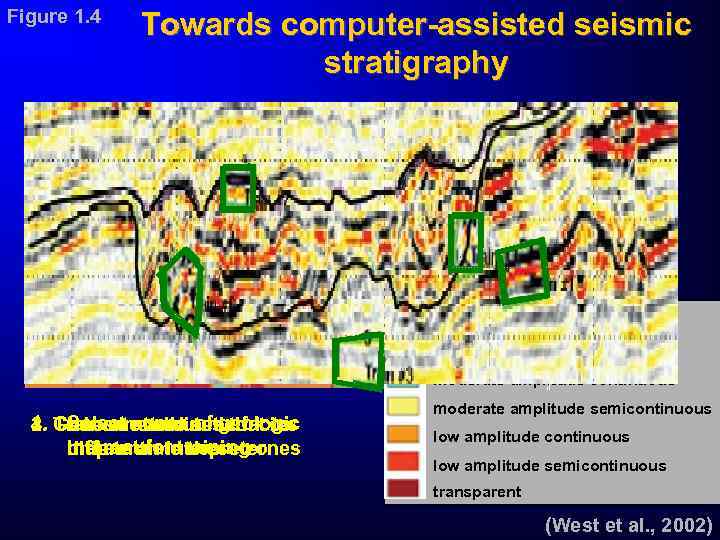
Figure 1. 4 Towards computer-assisted seismic stratigraphy high amplitude continuous high amplitude semicontinuous moderate amplitude continuous 1. Generate a seismic facies 4. Select attributes that 3. Train a zones of geologic 2. Chooseneural network to interestan interpreter map imitate for training differentiate these zones moderate amplitude semicontinuous low amplitude semicontinuous transparent (West et al. , 2002)
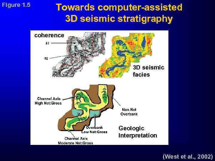
Figure 1. 5 Towards computer-assisted 3 D seismic stratigraphy coherence 3 D seismic facies Geologic Interpretation (West et al. , 2002)
A simple working definition A seismic attribute is any measure of seismic data that helps us better visualize or quantify features of interpretation interest. There are four main uses for seismic attributes…
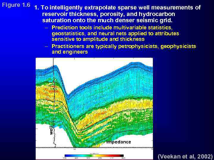
Figure 1. 6 1. To intelligently extrapolate sparse well measurements of reservoir thickness, porosity, and hydrocarbon saturation onto the much denser seismic grid. well – Prediction tools include multivariable statistics, geostatistics, and neural nets applied to attributes sensitive to amplitude and thickness – Practitioners are typically petrophysicists, geophysicists and engineers impedance (Veekan et al, 2002)
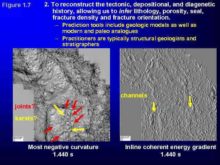
Figure 1. 7 2. To reconstruct the tectonic, depositional, and diagenetic history, allowing us to infer lithology, porosity, seal, fracture density and fracture orientation. – Prediction tools include geologic models as well as modern and paleo analogues – Practitioners are typically structural geologists and stratigraphers channels joints? karsts? Most negative curvature 1. 440 s Inline coherent energy gradient 1. 440 s
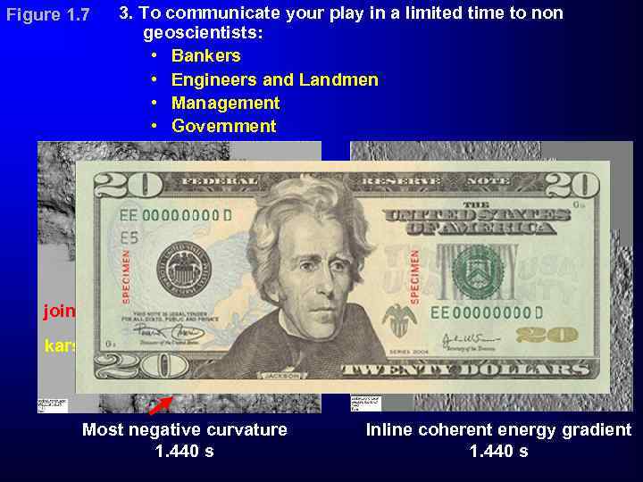
Figure 1. 7 3. To communicate your play in a limited time to non geoscientists: • Bankers • Engineers and Landmen • Management • Government channels joints? karsts? Most negative curvature 1. 440 s Inline coherent energy gradient 1. 440 s
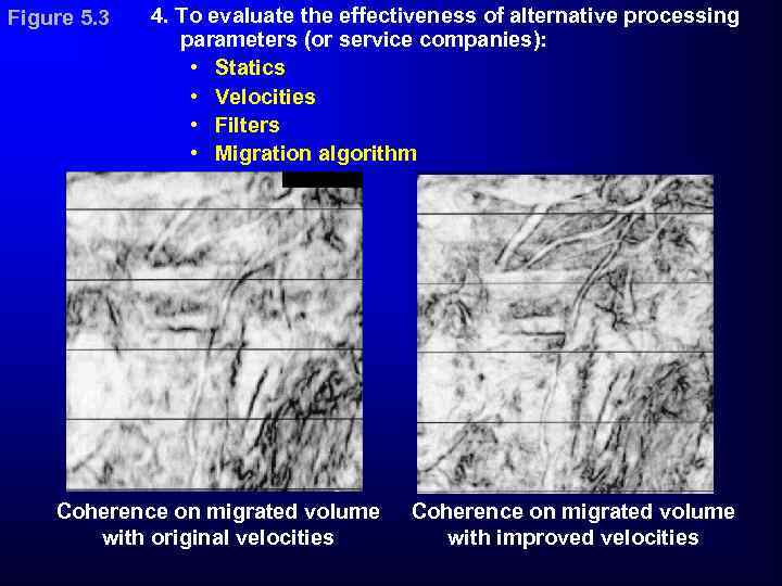
Figure 5. 3 4. To evaluate the effectiveness of alternative processing parameters (or service companies): • Statics • Velocities • Filters • Migration algorithm Coherence on migrated volume with original velocities Coherence on migrated volume with improved velocities
Quick Review of some Basic Building Blocks • The analytic trace • Complex trace attributes • Window-based attributes • Multiattribute color display
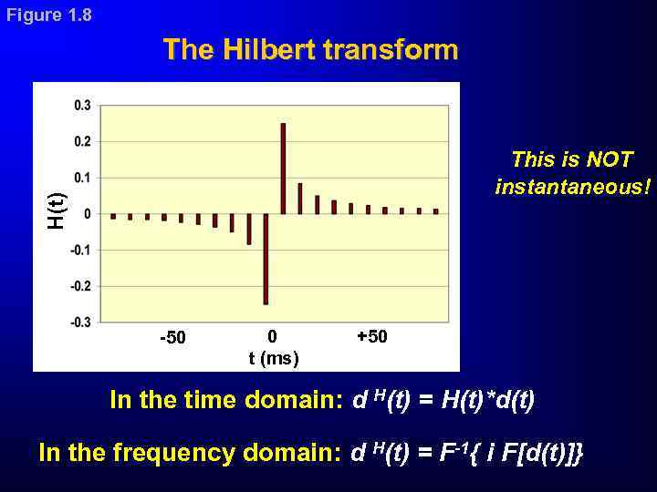
Figure 1. 8 The Hilbert transform H(t) This is NOT instantaneous! -50 0 t (ms) +50 In the time domain: d H(t) = H(t)*d(t) In the frequency domain: d H(t) = F-1{ i F[d(t)]}
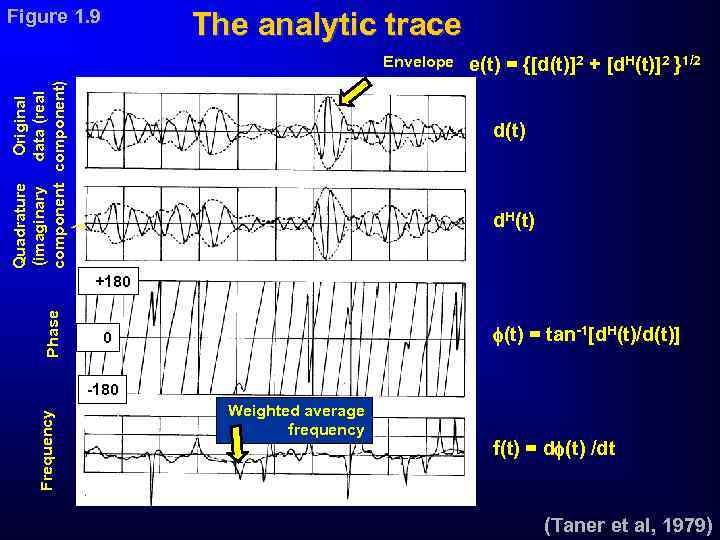
Figure 1. 9 The analytic trace Original Quadrature data (real (imaginary component) ) Envelope e(t) = {[d(t)]2 + [d. H(t)]2 }1/2 d(t) d. H(t) Phase +180 (t) = tan-1[d. H(t)/d(t)] 0 Frequency -180 Weighted average frequency f(t) = d (t) /dt (Taner et al, 1979)
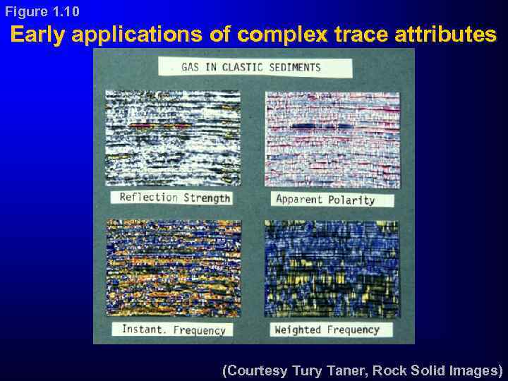
Figure 1. 10 Early applications of complex trace attributes (Courtesy Tury Taner, Rock Solid Images)
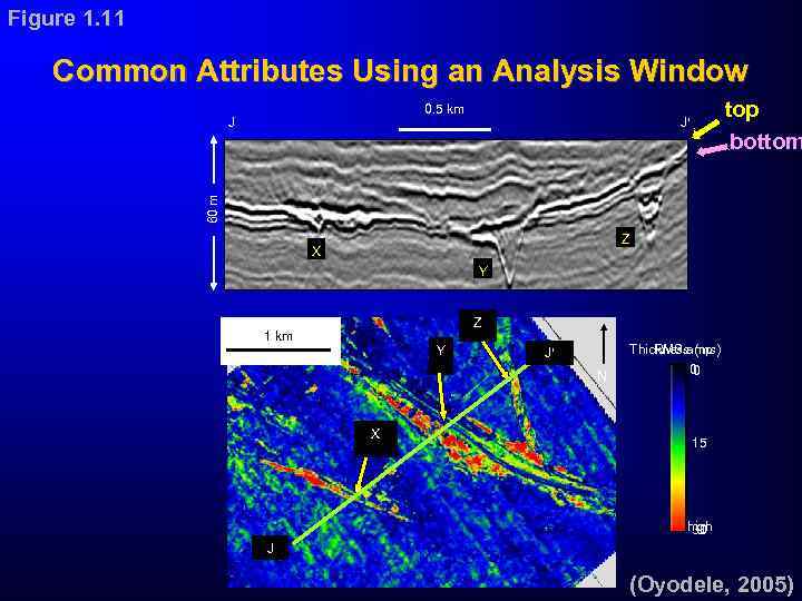
Figure 1. 11 Common Attributes Using an Analysis Window 0. 5 km top bottom J 60 m J Z X Y Z 1 km Y J N X Thickness (ms) RMS amp 0 0 15 high 30 J (Oyodele, 2005)
Course Outline Introduction Basic concepts Multiattribute display Spectral decomposition Geometric attributes Dip and azimuth Coherence Curvature and reflector shape Lateral changes in amplitude and pattern recognition Attributes and the seismic interpreter Structural deformation Clastic environments Carbonate environments Deep water deposition and drilling hazards Reservoir heterogeneity Issues and the seismic processor Influence of acquisition and processing Structure-oriented filtering and image enhancement Prestack geometric attributes
1 b: Multiattribute Display After this section you should be able to: • Identify good and bad color display practices, • Display multiple attributes in a single image, and • Apply color schemes that allow you to effectively communicate these features to others.
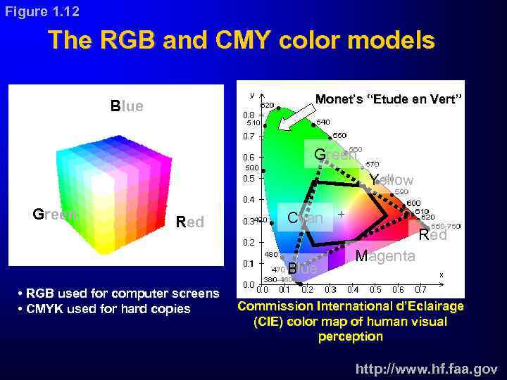
Figure 1. 12 The RGB and CMY color models Monet’s “Etude en Vert” Blue Green Yellow Green Red Cyan Blue • RGB used for computer screens • CMYK used for hard copies Red Magenta Commission International d’Eclairage (CIE) color map of human visual perception http: //www. hf. faa. gov
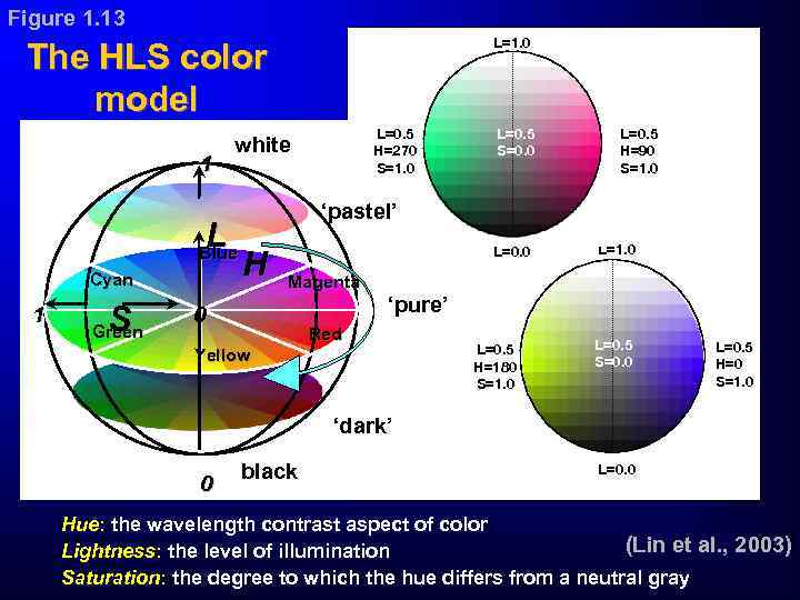
Figure 1. 13 L=1. 0 The HLS color model 1 L Blue Cyan 1 S Green L=0. 5 H=270 S=1. 0 white L=0. 5 S=0. 0 L=0. 5 H=90 S=1. 0 ‘pastel’ H L=0. 0 L=1. 0 Magenta ‘pure’ 0 Red Yellow L=0. 5 H=180 S=1. 0 L=0. 5 S=0. 0 L=0. 5 H=0 S=1. 0 ‘dark’ 0 black L=0. 0 Hue: the wavelength contrast aspect of color (Lin et al. , 2003) Lightness: the level of illumination Saturation: the degree to which the hue differs from a neutral gray
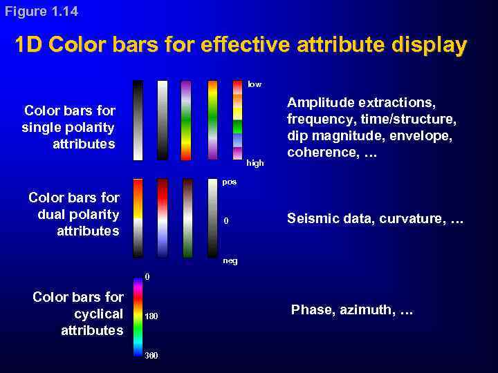
Figure 1. 14 1 D Color bars for effective attribute display low Color bars for single polarity attributes high Amplitude extractions, frequency, time/structure, dip magnitude, envelope, coherence, … pos Color bars for dual polarity attributes 0 Seismic data, curvature, … neg 0 Color bars for cyclical attributes 180 360 Phase, azimuth, …
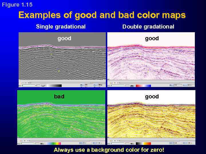
Figure 1. 15 Examples of good and bad color maps Single gradational good bad Double gradational good Always use a background color for zero!
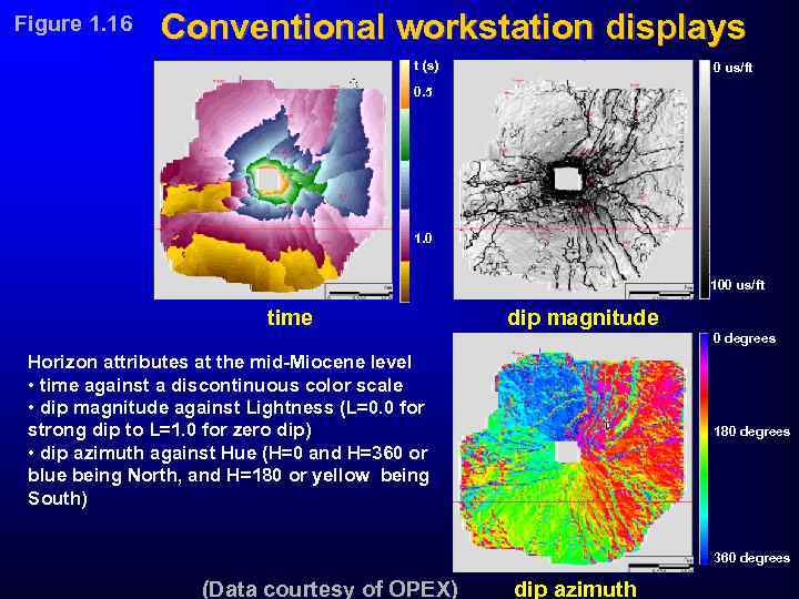
Figure 1. 16 Conventional workstation displays t (s) 0 us/ft 0. 5 1. 0 100 us/ft time dip magnitude 0 degrees Horizon attributes at the mid-Miocene level • time against a discontinuous color scale • dip magnitude against Lightness (L=0. 0 for strong dip to L=1. 0 for zero dip) • dip azimuth against Hue (H=0 and H=360 or blue being North, and H=180 or yellow being South) 180 degrees 360 degrees (Data courtesy of OPEX) dip azimuth
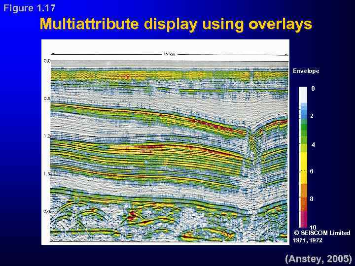
Figure 1. 17 Multiattribute display using overlays Envelope 0 2 4 6 8 10 © SEISCOM Limited 1971, 1972 (Anstey, 2005)
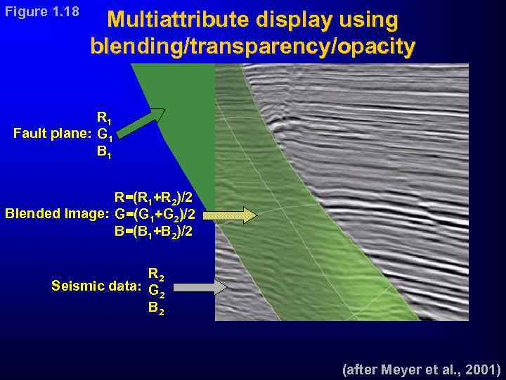
Figure 1. 18 Multiattribute display using blending/transparency/opacity R 1 Fault plane: G 1 B 1 R=(R 1+R 2)/2 Blended Image: G=(G 1+G 2)/2 B=(B 1+B 2)/2 R 2 Seismic data: G 2 B 2 (after Meyer et al. , 2001)
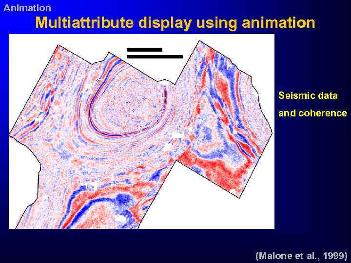
Animation Multiattribute display using animation Seismic data and coherence (Maione et al. , 1999)
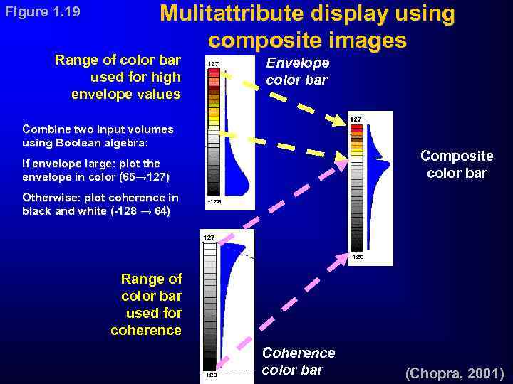
Figure 1. 19 Mulitattribute display using composite images Range of color bar used for high envelope values Envelope color bar Combine two input volumes using Boolean algebra: Composite color bar If envelope large: plot the envelope in color (65→ 127) Otherwise: plot coherence in black and white (-128 → 64) Range of color bar used for coherence Coherence color bar (Chopra, 2001)
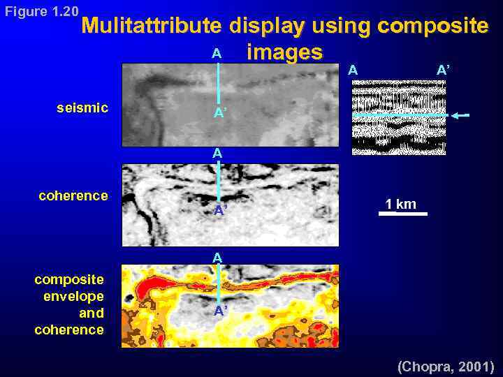
Figure 1. 20 Mulitattribute display using composite A images A seismic A’ A’ A coherence A’ 1 km A composite envelope and coherence A’ (Chopra, 2001)
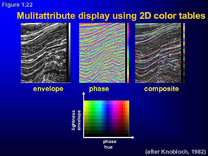
Figure 1. 22 Mulitattribute display using 2 D color tables phase composite lightness envelope phase hue (after Knobloch, 1982)
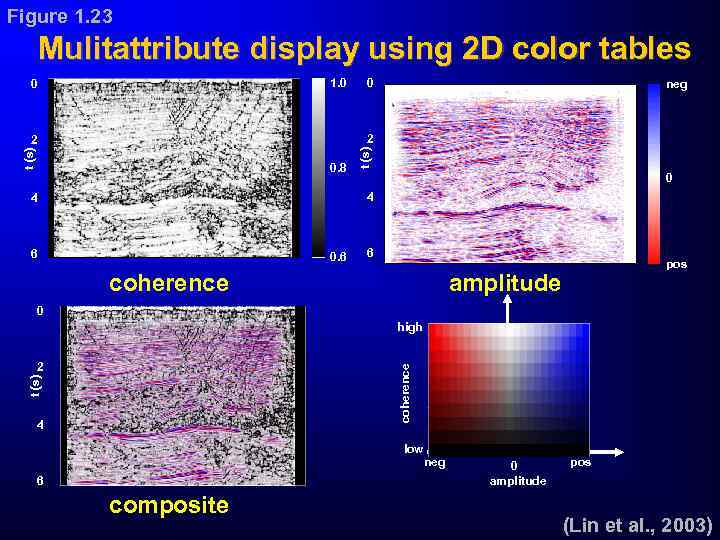
Figure 1. 23 Mulitattribute display using 2 D color tables 1. 0 0 0 neg t (s) 0. 8 t (s) 2 2 0 4 4 6 0. 6 6 coherence pos amplitude 0 high t (s) coherence 2 4 low 6 composite neg 0 amplitude pos (Lin et al. , 2003)
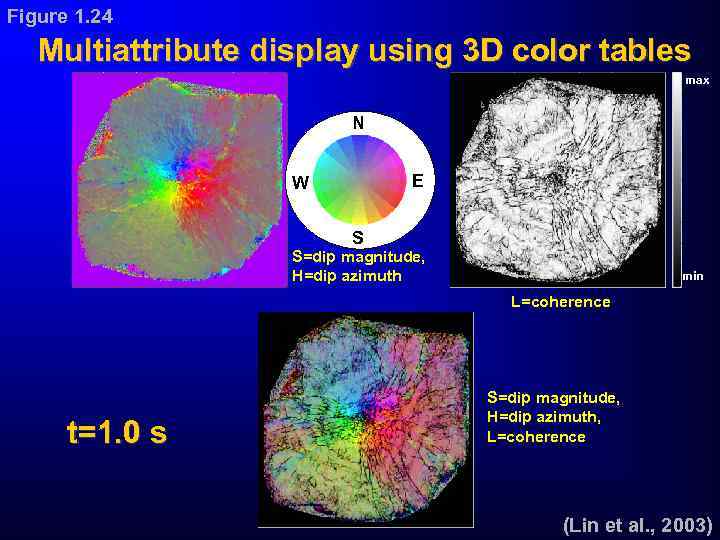
Figure 1. 24 Multiattribute display using 3 D color tables max N E W S S=dip magnitude, H=dip azimuth min L=coherence t=1. 0 s S=dip magnitude, H=dip azimuth, L=coherence (Lin et al. , 2003)
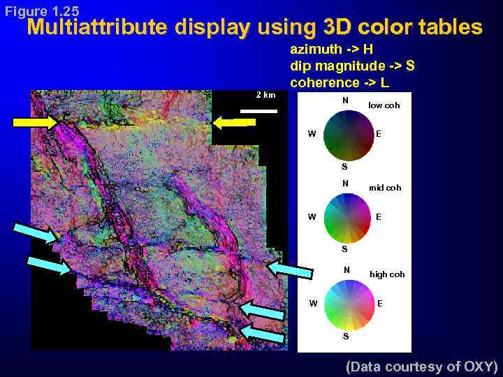
Figure 1. 25 Multiattribute display using 3 D color tables 2 km azimuth -> H dip magnitude -> S coherence -> L N W low coh E S N W mid coh E S N W high coh E S (Data courtesy of OXY)
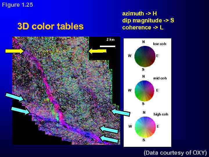
Figure 1. 25 azimuth -> H dip magnitude -> S coherence -> L 3 D color tables 2 km N W low coh E S N W mid coh E S N W high coh E S (Data courtesy of OXY)
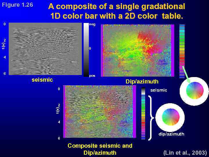
Figure 1. 26 A composite of a single gradational 1 D color bar with a 2 D color table. 0 neg t (s) 2 0 4 6 pos seismic N Dip/azimuth 0 seismic E W S 2 t (s) N W 4 E S dip/azimuth 6 Composite seismic and Dip/azimuth (Lin et al. , 2003)
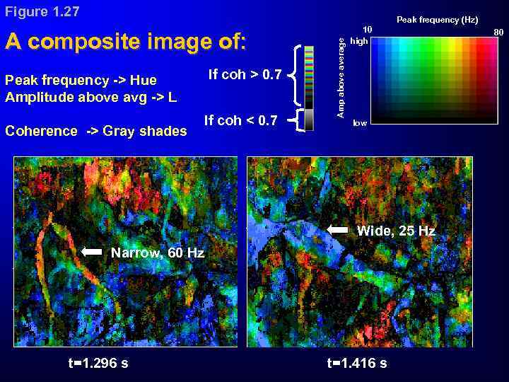
Figure 1. 27 A composite image of: If coh > 0. 7 Peak frequency -> Hue Amplitude above avg -> L Coherence -> Gray shades If coh < 0. 7 Amp above average Peak frequency (Hz) 10 high low Wide, 25 Hz Narrow, 60 Hz t=1. 296 s t=1. 416 s 80
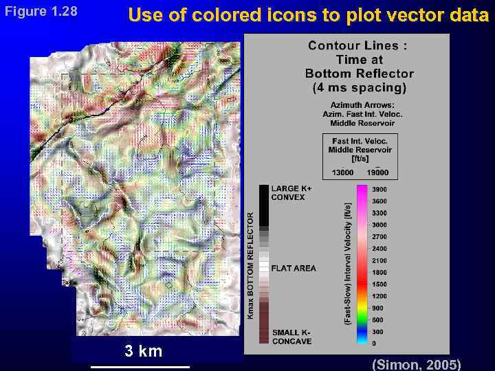
Figure 1. 28 Use of colored icons to plot vector data 3 km (Simon, 2005)
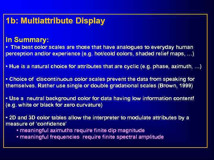
1 b: Multiattribute Display In Summary: • The best color scales are those that have analogues to everyday human perception and/or experience (e. g. hot/cold colors, shaded relief maps, …) • Hue is a natural choice for attributes that are cyclic (e. g. phase, azimuth, …) • Choice of discontinuous color scales prevent the data from speaking for themselves. Rather use single or double gradational scales (Brown, 1999) • Use a neutral background color for data having low information content! (e. g. white or black for zero curvature) • 2 D and 3 D color tables allow the interpreter to modulate attributes by a measure of ‘confidence’ • meaningful azimuths require finite dip magnitude • meaningful frequencies require finite spectral amplitude
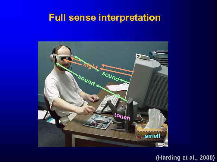
Full sense interpretation sigh t so un d sou nd touc h smell (Harding et al. , 2000)
Marfurt K. 1 - Introduction.ppt