Sedimentological facies models versus digital reservoir models How

Sedimentological facies models versus digital reservoir models. How do they relate?

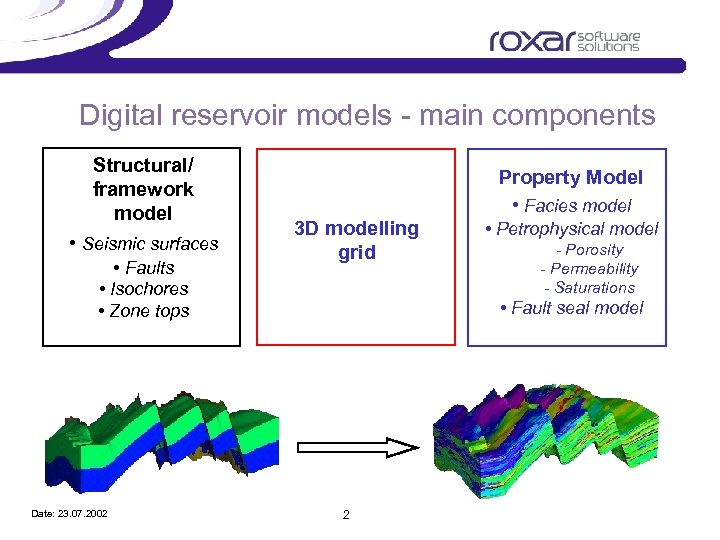Digital reservoir models - main components Structural/ framework model • Seismic surfaces • Faults • Isochores • Zone tops Date: 23. 07. 2002 Property Model • Facies model 3 D modelling grid • Petrophysical model - Porosity - Permeability - Saturations • Fault seal model 2

Role of geological interpretations and conceptual models Critical role through entire modelling process Zonation Building of modelling grid Choice of facies modelling techniques Input parameters to facies modelling. . . Date: 23. 07. 2002 3

Reservoir zonation for 3 D modelling General rule is that zonation should follow time lines. Lithostratigraphic zonations are often OK for volumetric calculations. BUT are often unsuitable for building flow simulation models. Date: 23. 07. 2002 4

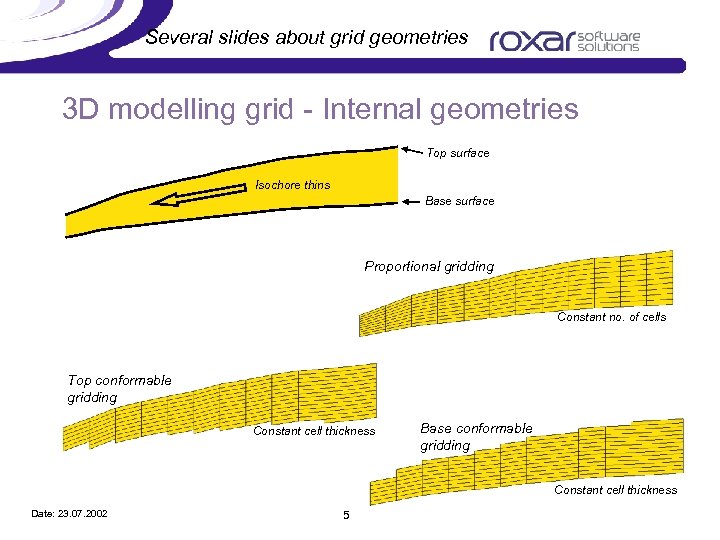Several slides about grid geometries 3 D modelling grid - Internal geometries Top surface Isochore thins Base surface Proportional gridding Constant no. of cells Top conformable gridding Constant cell thickness Base conformable gridding Constant cell thickness Date: 23. 07. 2002 5

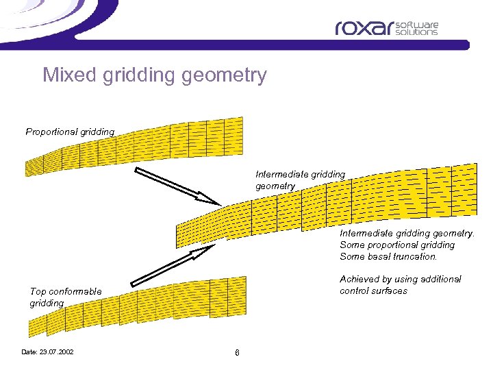Mixed gridding geometry Proportional gridding Intermediate gridding geometry. Some proportional gridding Some basal truncation. Achieved by using additional control surfaces Top conformable gridding Date: 23. 07. 2002 6

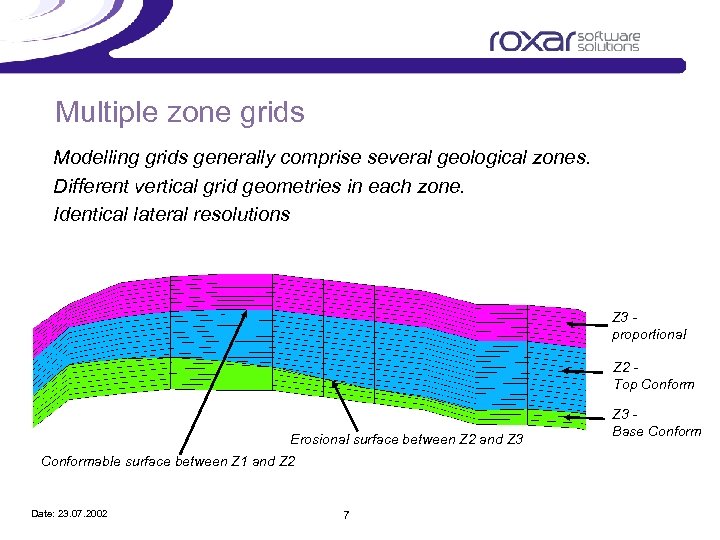Multiple zone grids Modelling grids generally comprise several geological zones. Different vertical grid geometries in each zone. Identical lateral resolutions Z 3 proportional Z 2 Top Conform Erosional surface between Z 2 and Z 3 Conformable surface between Z 1 and Z 2 Date: 23. 07. 2002 7 Z 3 Base Conform

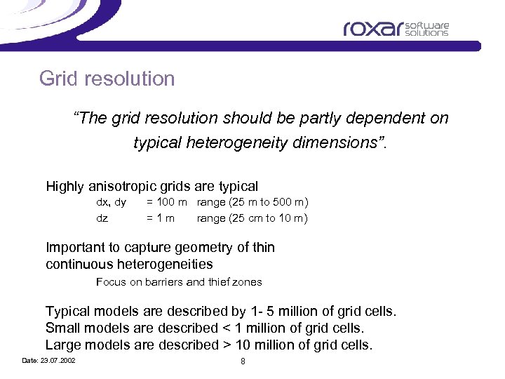Grid resolution “The grid resolution should be partly dependent on typical heterogeneity dimensions”. Highly anisotropic grids are typical dx, dy dz = 100 m range (25 m to 500 m) =1 m range (25 cm to 10 m) Important to capture geometry of thin continuous heterogeneities Focus on barriers and thief zones Typical models are described by 1 - 5 million of grid cells. Small models are described < 1 million of grid cells. Large models are described > 10 million of grid cells. Date: 23. 07. 2002 8

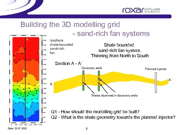Building the 3 D modelling grid - sand-rich fan systems A Isochore shale-bounded sand-rich fan. Shale bounded sand-rich fan system. Thinning from North to South Section A - A` Discovery wells Planned injector A` A Shales observed in discovery wells A` Date: 23. 07. 2002 Q 1 - How should the modelling grid be built? Q 2 - What is the shale geometry towards the planned injector? 9

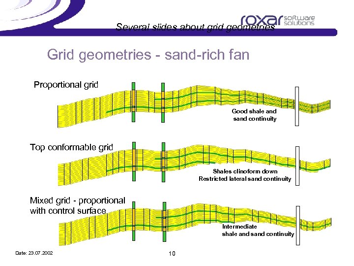Several slides about grid geometries Grid geometries - sand-rich fan Proportional grid Good shale and sand continuity Top conformable grid Shales clinoform down Restricted lateral sand continuity Mixed grid - proportional with control surface Intermediate shale and sand continuity Date: 23. 07. 2002 10

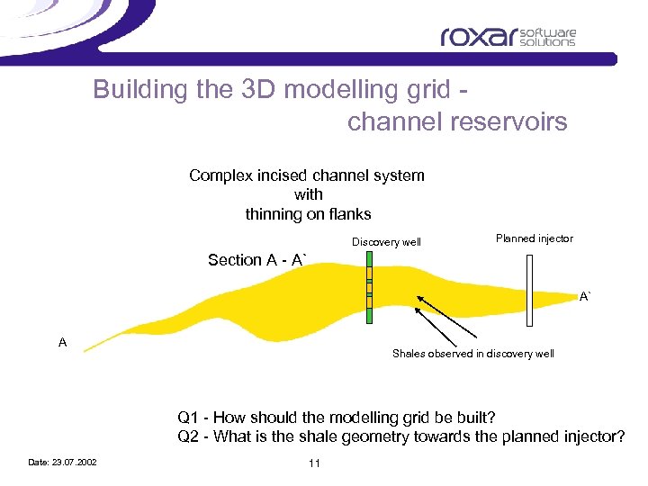Building the 3 D modelling grid channel reservoirs Complex incised channel system with thinning on flanks Discovery well Planned injector Section A - A` A` A Shales observed in discovery well Q 1 - How should the modelling grid be built? Q 2 - What is the shale geometry towards the planned injector? Date: 23. 07. 2002 11

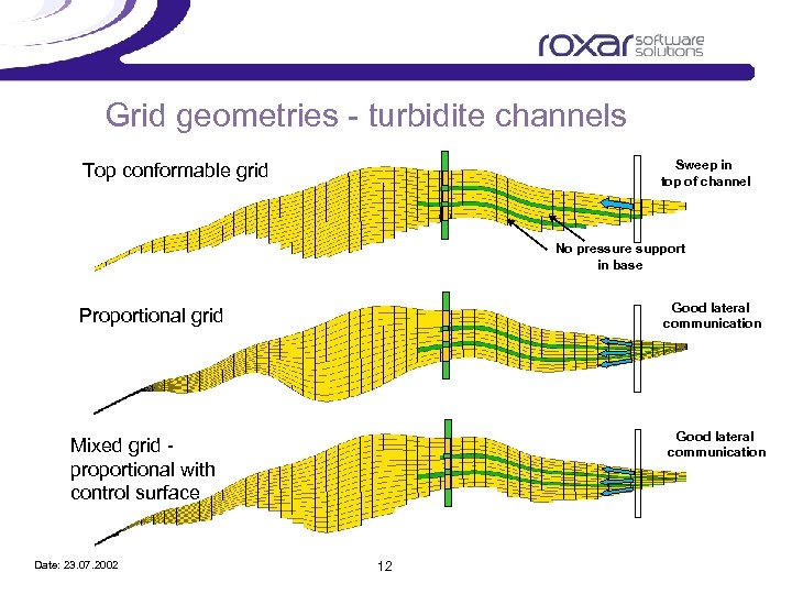Grid geometries - turbidite channels Sweep in top of channel Top conformable grid No pressure support in base Good lateral communication Proportional grid Good lateral communication Mixed grid proportional with control surface Date: 23. 07. 2002 12

Approaches for property modelling in 3 D grid 1) Direct modelling of petrophysics 2) Build facies model first and constrain petrophysics to facies model. Date: 23. 07. 2002 13

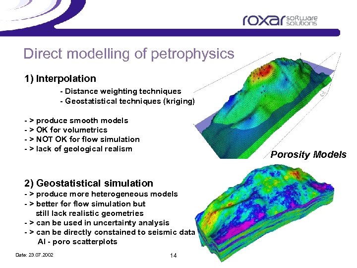Direct modelling of petrophysics 1) Interpolation - Distance weighting techniques - Geostatistical techniques (kriging) - > produce smooth models - > OK for volumetrics - > NOT OK for flow simulation - > lack of geological realism Porosity Models 2) Geostatistical simulation - > produce more heterogeneous models - > better for flow simulation but still lack realistic geometries - > can be used in uncertainty analysis - > can be directly constained to seismic data AI - poro scatterplots Date: 23. 07. 2002 14

Facies modelling approaches 1) Facies and body definition from seismic 2) Manual digitising of facies 3) Geostatistical/Stochastic techniques 4) Process based mathematical models Date: 23. 07. 2002 15

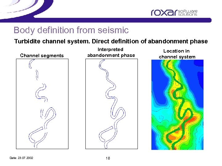Body definition from seismic Turbidite channel system. Direct definition of abandonment phase Channel segments Date: 23. 07. 2002 Interpreted abandonment phase 16 Location in channel system

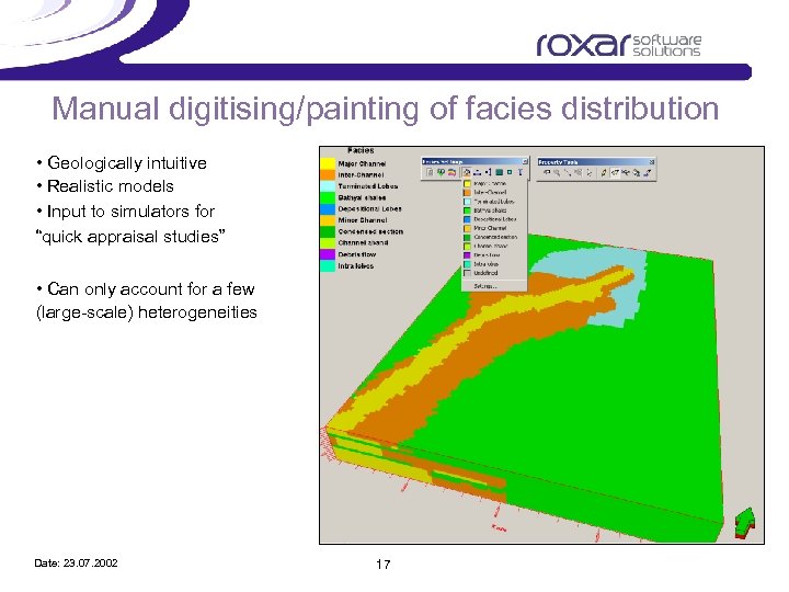Manual digitising/painting of facies distribution • Geologically intuitive • Realistic models • Input to simulators for “quick appraisal studies” • Can only account for a few (large-scale) heterogeneities Date: 23. 07. 2002 17

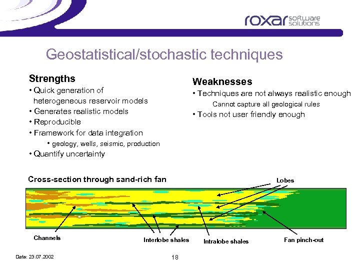Geostatistical/stochastic techniques Strengths Weaknesses • Quick generation of heterogeneous reservoir models • Generates realistic models • Reproducible • Framework for data integration • geology, wells, seismic, production • Quantify uncertainty • Techniques are not always realistic enough Cannot capture all geological rules • Tools not user friendly enough Cross-section through sand-rich fan Channels Date: 23. 07. 2002 Lobes Interlobe shales 18 Intralobe shales Fan pinch-out

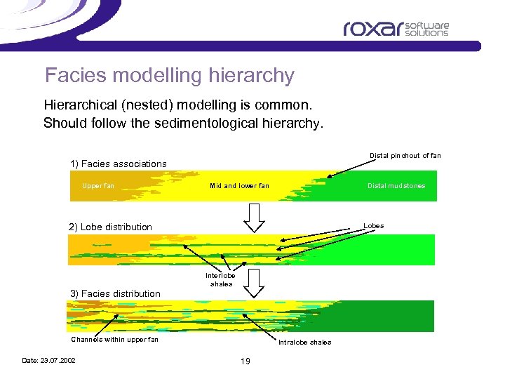Facies modelling hierarchy Hierarchical (nested) modelling is common. Should follow the sedimentological hierarchy. Distal pinchout of fan 1) Facies associations Upper fan Distal mudstones Mid and lower fan 2) Lobe distribution 3) Facies distribution Lobes Interlobe shales Channels within upper fan Date: 23. 07. 2002 Intralobe shales 19

Facies models Stochastic models Use equations and statistics to describe geometries Challenge is to find the appropriate equations and statistics Has been a tendency to try to make the geology pass in with the mathematics BUT Basis for an appropriate stochastic model should be a well defined conceptual geological model. Date: 23. 07. 2002 20

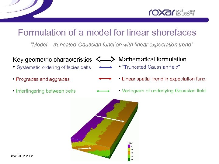Formulation of a model for linear shorefaces “Model = truncated Gaussian function with linear expectation trend” Key geometric characteristics • Systematic ordering of facies belts Mathematical formulation • “Truncated Gaussian field” • Progrades and aggrades • Linear spatial trend in expectation func. • Interfingering between belts • Variogram of underlying Gaussian field Date: 23. 07. 2002 21

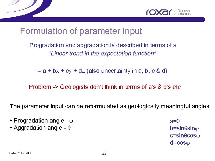Formulation of parameter input Progradation and aggradation is described in terms of a “Linear trend in the expectation function” = a + bx + cy + dz (also uncertainty in a, b, c & d) Problem -> Geologists don’t think in terms of a’s & b’s etc The parameter input can be reformulated as geologically meaningful angles • Progradation angle - j • Aggradation angle - q Date: 23. 07. 2002 a=0, b=sinqsinj c=sinqcosj d=cosj 22

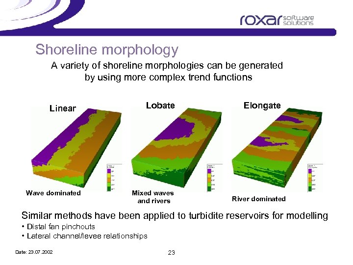Shoreline morphology A variety of shoreline morphologies can be generated by using more complex trend functions Linear Wave dominated Lobate Mixed waves and rivers Elongate River dominated Similar methods have been applied to turbidite reservoirs for modelling • Distal fan pinchouts • Lateral channel/levee relationships Date: 23. 07. 2002 23

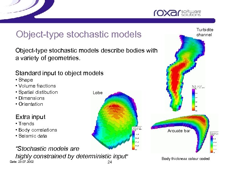Turbidite channel Object-type stochastic models describe bodies with a variety of geometries. Standard input to object models • Shape • Volume fractions • Spatial distibution • Dimensions • Orientation Lobe Extra input • Trends • Body correlations • Seismic data Arcuate bar “Stochastic models are highly constrained by deterministic input” Date: 23. 07. 2002 24 Body thickness colour coded

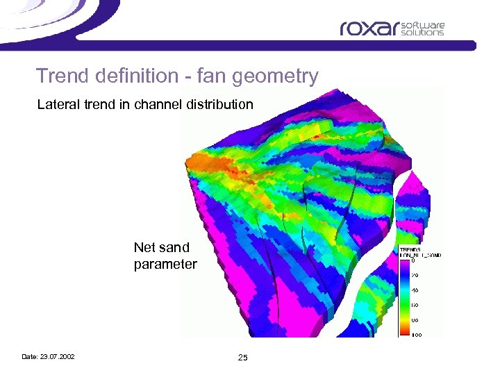Trend definition - fan geometry Lateral trend in channel distribution Net sand parameter Date: 23. 07. 2002 25

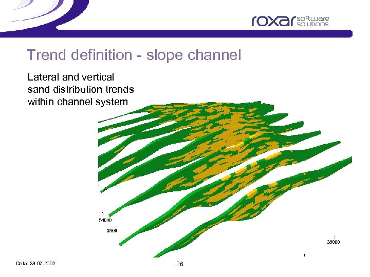Trend definition - slope channel Lateral and vertical sand distribution trends within channel system Date: 23. 07. 2002 26

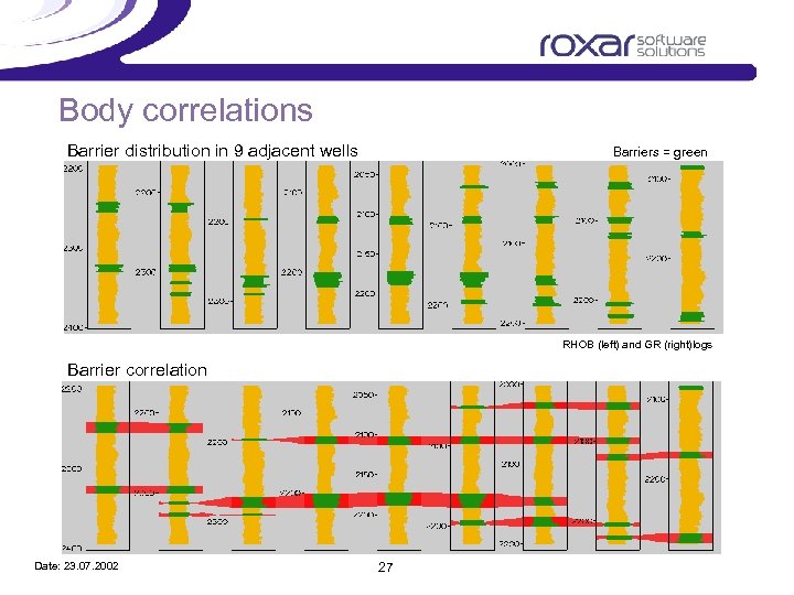Body correlations Barrier distribution in 9 adjacent wells Barriers = green RHOB (left) and GR (right)logs Barrier correlation Date: 23. 07. 2002 27

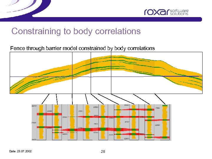Constraining to body correlations Fence through barrier model constrained by body correlations Date: 23. 07. 2002 28

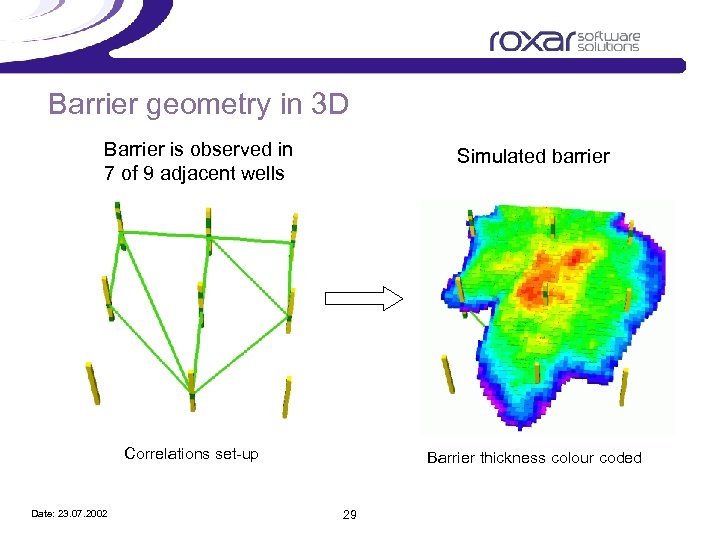Barrier geometry in 3 D Barrier is observed in 7 of 9 adjacent wells Simulated barrier Correlations set-up Date: 23. 07. 2002 Barrier thickness colour coded 29

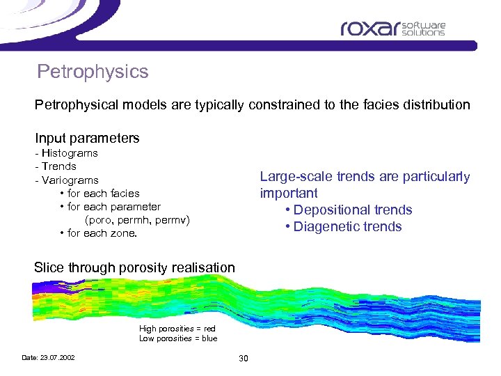Petrophysics Petrophysical models are typically constrained to the facies distribution Input parameters - Histograms - Trends - Variograms • for each facies • for each parameter (poro, permh, permv) • for each zone. Large-scale trends are particularly important • Depositional trends • Diagenetic trends Slice through porosity realisation High porosities = red Low porosities = blue Date: 23. 07. 2002 30

Role of geology/geologist in 3 D reservoir modelling Zonation Input parameters to facies modelling • Time lines • Major (continuous heterogneities) • Dimensions/orientation etc Integration with other disciplines Building of modelling grid • Correct internal geometries should be • Geophysics • Reservoir technology conformable with time lines Choice of facies modelling techniques Date: 23. 07. 2002 QC 31

Some important challenges Optimal use of seismic data Direct body extraction Modelling of thin continuous shales Often difficult to capture in reservoir simulator Conceptual models and internal architecture of slope channel systems Flexible modelling of compensational features Date: 23. 07. 2002 32