Section 7 -5 Testing a Claim About a

Section 7 -5 Testing a Claim About a Mean: Not Known Created by Erin Hodgess, Houston, Texas

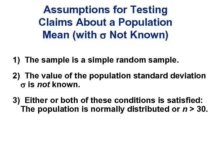
Assumptions for Testing Claims About a Population Mean (with Not Known) 1) The sample is a simple random sample. 2) The value of the population standard deviation is not known. 3) Either or both of these conditions is satisfied: The population is normally distributed or n > 30.

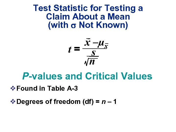
Test Statistic for Testing a Claim About a Mean (with Not Known) x –µx t= s n P-values and Critical Values v Found in Table A-3 v Degrees of freedom (df) = n – 1

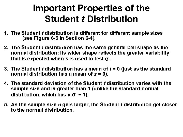
Important Properties of the Student t Distribution 1. The Student t distribution is different for different sample sizes (see Figure 6 -5 in Section 6 -4). 2. The Student t distribution has the same general bell shape as the normal distribution; its wider shape reflects the greater variability that is expected when s is used to test . 3. The Student t distribution has a mean of t = 0 (just as the standard normal distribution has a mean of z = 0). 4. The standard deviation of the Student t distribution varies with the sample size and is greater than 1 (unlike the standard normal distribution, which has a = 1). 5. As the sample size n gets larger, the Student t distribution get closer to the normal distribution.

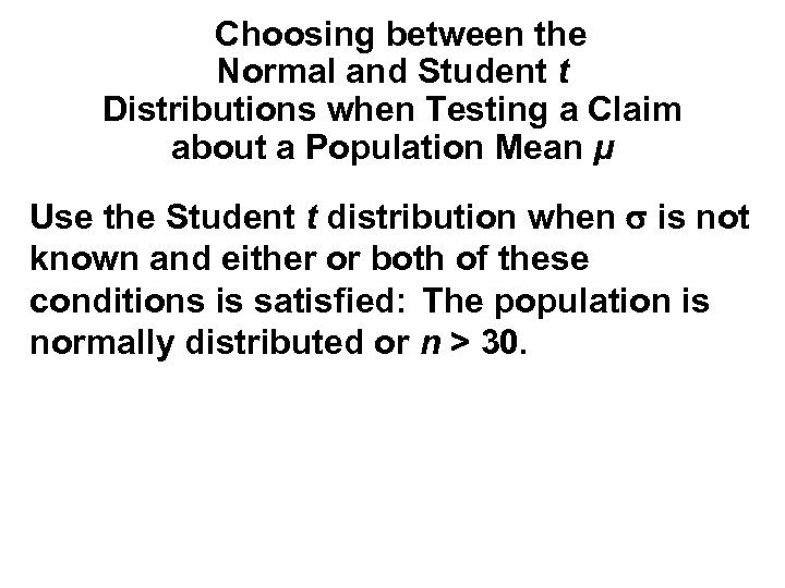
Choosing between the Normal and Student t Distributions when Testing a Claim about a Population Mean µ Use the Student t distribution when is not known and either or both of these conditions is satisfied: The population is normally distributed or n > 30.

Example: A premed student in a statistics class is required to do a class project. She plans to collect her own sample data to test the claim that the mean body temperature is less than 98. 6°F. After carefully planning a procedure for obtaining a simple random sample of 12 healthy adults, she measures their body temperatures and obtains the results on page 409. Use a 0. 05 significance level to test the claim these body temperatures come from a population with a mean that is less than 98. 6°F. Use the Traditional method. There are no outliers, and based on a histogram and normal quantile plot, we can assume that the data are from a population with a normal distribution. We use the sample data to find n = 12, x = 98. 39, and s = 0. 535.

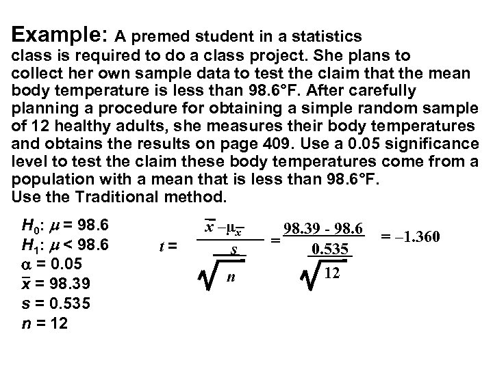
Example: A premed student in a statistics class is required to do a class project. She plans to collect her own sample data to test the claim that the mean body temperature is less than 98. 6°F. After carefully planning a procedure for obtaining a simple random sample of 12 healthy adults, she measures their body temperatures and obtains the results on page 409. Use a 0. 05 significance level to test the claim these body temperatures come from a population with a mean that is less than 98. 6°F. Use the Traditional method. H 0: = 98. 6 H 1: < 98. 6 = 0. 05 x = 98. 39 s = 0. 535 n = 12 t= x –µx s n 98. 39 - 98. 6 = 0. 535 12 = – 1. 360

Example: A premed student in a statistics class is required to do a class project. She plans to collect her own sample data to test the claim that the mean body temperature is less than 98. 6°F. After carefully planning a procedure for obtaining a simple random sample of 12 healthy adults, she measures their body temperatures and obtains the results on page 409. Use a 0. 05 significance level to test the claim these body temperatures come from a population with a mean that is less than 98. 6°F. Use the Traditional method. H 0: = 98. 6 H 1: < 98. 6 = 0. 05 x = 98. 39 s = 0. 535 n = 12 t = – 1. 360 Because the test statistic of t = – 1. 360 does not fall in the critical region, we fail to reject H 0. There is not sufficient evidence to to support the claim that the sample comes from a population with a mean less than 98. 6°F.

The larger Student t critical value shows that with a small sample, the sample evidence must be more extreme before we consider the difference is significant.

P-Value Method v. Table A-3 includes only selected values of . v. Specific P-values usually cannot be found. v. Use Table to identify limits that contain the P-value. v. Some calculators and computer programs will find exact P-values.

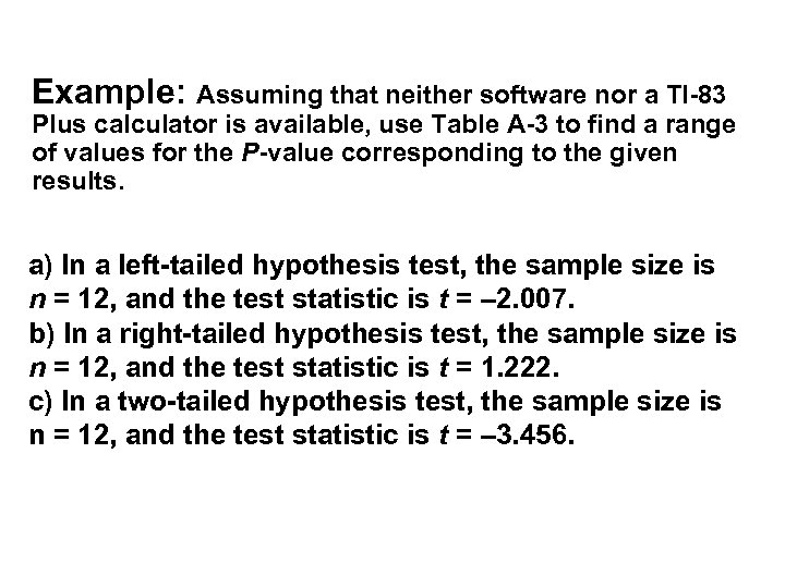
Example: Assuming that neither software nor a TI-83 Plus calculator is available, use Table A-3 to find a range of values for the P-value corresponding to the given results. a) In a left-tailed hypothesis test, the sample size is n = 12, and the test statistic is t = – 2. 007. b) In a right-tailed hypothesis test, the sample size is n = 12, and the test statistic is t = 1. 222. c) In a two-tailed hypothesis test, the sample size is n = 12, and the test statistic is t = – 3. 456.

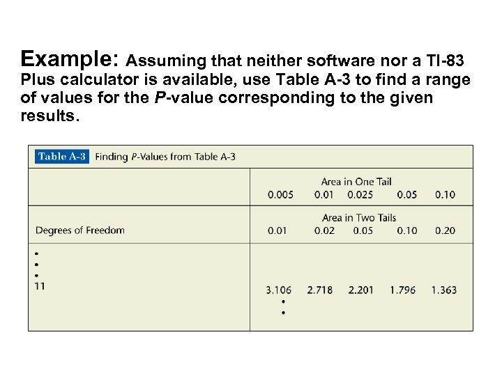
Example: Assuming that neither software nor a TI-83 Plus calculator is available, use Table A-3 to find a range of values for the P-value corresponding to the given results.

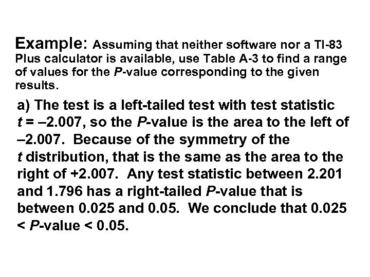
Example: Assuming that neither software nor a TI-83 Plus calculator is available, use Table A-3 to find a range of values for the P-value corresponding to the given results. a) The test is a left-tailed test with test statistic t = – 2. 007, so the P-value is the area to the left of – 2. 007. Because of the symmetry of the t distribution, that is the same as the area to the right of +2. 007. Any test statistic between 2. 201 and 1. 796 has a right-tailed P-value that is between 0. 025 and 0. 05. We conclude that 0. 025 < P-value < 0. 05.

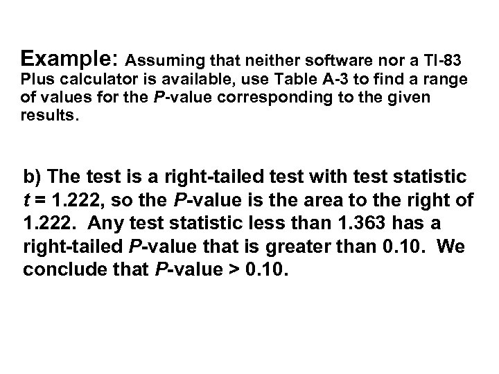
Example: Assuming that neither software nor a TI-83 Plus calculator is available, use Table A-3 to find a range of values for the P-value corresponding to the given results. b) The test is a right-tailed test with test statistic t = 1. 222, so the P-value is the area to the right of 1. 222. Any test statistic less than 1. 363 has a right-tailed P-value that is greater than 0. 10. We conclude that P-value > 0. 10.

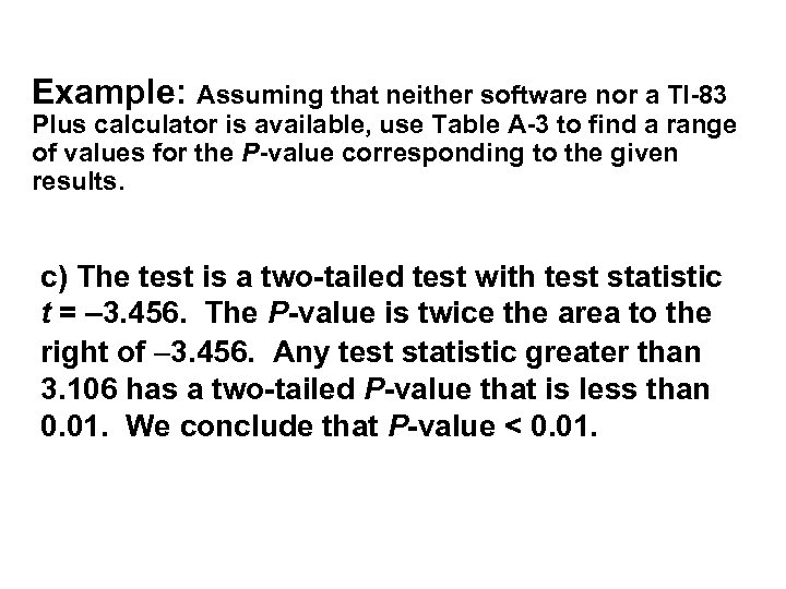
Example: Assuming that neither software nor a TI-83 Plus calculator is available, use Table A-3 to find a range of values for the P-value corresponding to the given results. c) The test is a two-tailed test with test statistic t = – 3. 456. The P-value is twice the area to the right of – 3. 456. Any test statistic greater than 3. 106 has a two-tailed P-value that is less than 0. 01. We conclude that P-value < 0. 01.