c9ac1616f1164496d9a05db1ea321b3e.ppt
- Количество слайдов: 73

Searching and Integrating Information on the Web Seminar 3: Data Cleansing Professor Chen Li UC Irvine 1
Paper readings • Efficient merge and purge: Hernandez and Stolfo, SIGMOD 1995 • Approximate String Joins in a Database (Almost) for Free, Gravano et al, VLDB 2001, • Efficient Record Linkage in Large Data Sets, Liang Jin, Chen Li, Sharad Mehrotra, DASFAA, 2003 • Sunita Sarawagi Anuradha Bhamidipaty, Interactive Deduplication Using Active Learning. Sarawagi and Bhamidipaty, KDD 2003 Seminar 3 2
Motivation • Correlate data from different data sources (e. g. , data integration) – Data is often dirty – Needs to be cleansed before being used • Example: – A hospital needs to merge patient records from different data sources – They have different formats, typos, and abbreviations Seminar 3 3
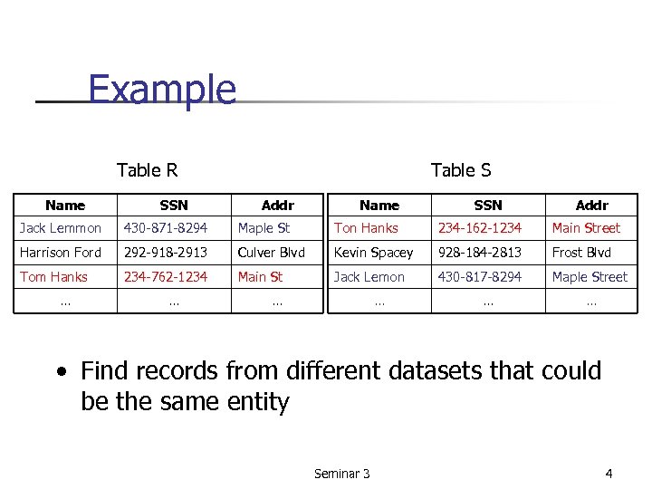
Example Table R Name SSN Table S Addr Name SSN Addr Jack Lemmon 430 -871 -8294 Maple St Ton Hanks 234 -162 -1234 Main Street Harrison Ford 292 -918 -2913 Culver Blvd Kevin Spacey 928 -184 -2813 Frost Blvd Tom Hanks 234 -762 -1234 Main St Jack Lemon 430 -817 -8294 Maple Street … … … • Find records from different datasets that could be the same entity Seminar 3 4
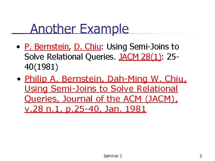
Another Example • P. Bernstein, D. Chiu: Using Semi-Joins to Solve Relational Queries. JACM 28(1): 2540(1981) • Philip A. Bernstein, Dah-Ming W. Chiu, Using Semi-Joins to Solve Relational Queries, Journal of the ACM (JACM), v. 28 n. 1, p. 25 -40, Jan. 1981 Seminar 3 5
Record linkage Problem statement: “Given two relations, identify the potentially matched records – Efficiently and – Effectively” Seminar 3 6
Challenges • How to define good similarity functions? – Many functions proposed (edit distance, cosine similarity, …) – Domain knowledge is critical § Names: “Wall Street Journal” and “LA Times” § Address: “Main Street” versus “Main St” • How to do matching efficiently – Offline join version – Online (interactive) search § Nearest search § Range search Seminar 3 7
Outline • Supporting string-similarity joins using RDBMS • Using mapping techniques • Interactive deduplication Seminar 3 8
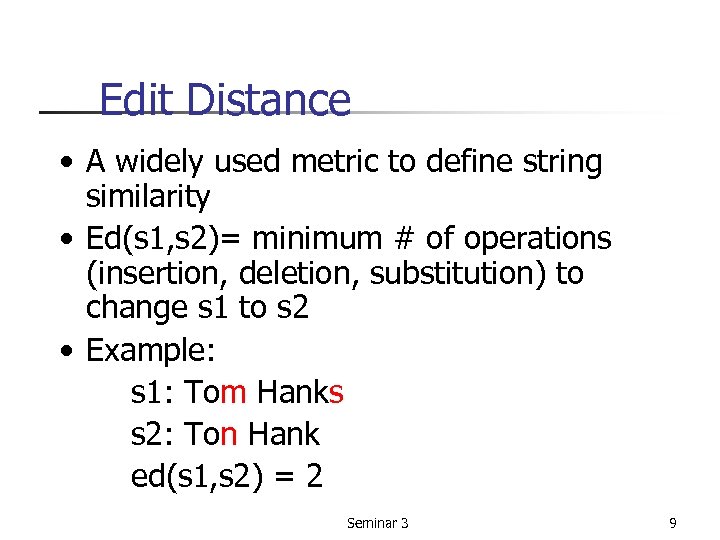
Edit Distance • A widely used metric to define string similarity • Ed(s 1, s 2)= minimum # of operations (insertion, deletion, substitution) to change s 1 to s 2 • Example: s 1: Tom Hanks s 2: Ton Hank ed(s 1, s 2) = 2 Seminar 3 9
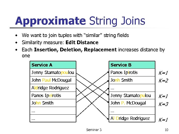
Approximate String Joins • We want to join tuples with “similar” string fields • Similarity measure: Edit Distance • Each Insertion, Deletion, Replacement increases distance by one Service A Service B Jenny Stamatopoulou Panos Ipirotis John Paul Mc. Dougal Jonh Smith Aldridge Rodriguez … Panos Ipeirotis Jenny Stamatopulou John Smith John P. Mc. Dougal … … … Al Dridge Rodriguez Seminar 3 K=1 K=2 K=1 K=3 K=1 10
Focus: Approximate String Joins over Relational DBMSs • Join two tables on string attributes and keep all pairs of strings with Edit Distance ≤ K • Solve the problem in a database-friendly way (if possible with an existing "vanilla" RDBMS) Seminar 3 11
Current Approaches for Processing Approximate String Joins No native support for approximate joins in RDBMSs Two existing (straightforward) solutions: • Join data outside of DBMS • Join data via user-defined functions (UDFs) inside the DBMS Seminar 3 12
Approximate String Joins outside of a DBMS 1. Export data 2. Join outside of DBMS 3. Import the result Main advantage: We can exploit any state-of-the-art string-matching algorithm, without restrictions from DBMS functionality Disadvantages: • Substantial amounts of data to be exported/imported • Cannot be easily integrated with further processing steps in the DBMS Seminar 3 13
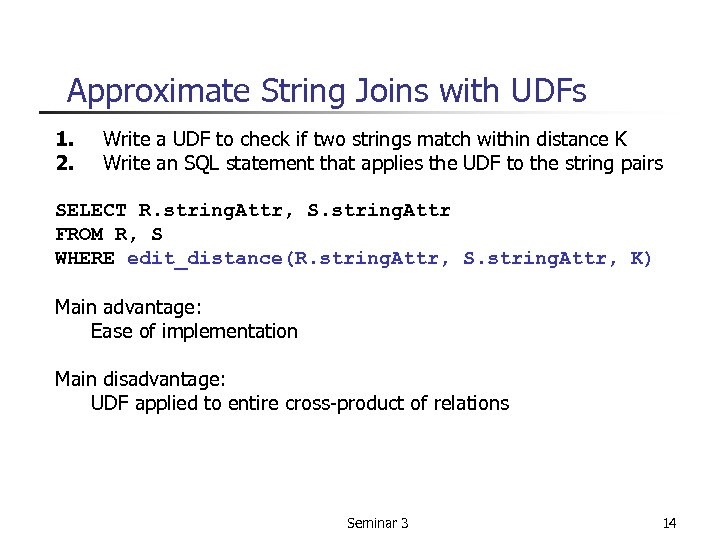
Approximate String Joins with UDFs 1. 2. Write a UDF to check if two strings match within distance K Write an SQL statement that applies the UDF to the string pairs SELECT R. string. Attr, S. string. Attr FROM R, S WHERE edit_distance(R. string. Attr, S. string. Attr, K) Main advantage: Ease of implementation Main disadvantage: UDF applied to entire cross-product of relations Seminar 3 14
Our Approach: Approximate String Joins over an Unmodified RDBMS 1. Preprocess data and generate auxiliary tables 2. Perform join exploiting standard RDBMS capabilities Advantages • No modification of underlying RDBMS needed. • Can leverage the RDBMS query optimizer. • Much more efficient than the approach based on naive UDFs Seminar 3 15
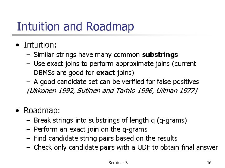
Intuition and Roadmap • Intuition: – Similar strings have many common substrings – Use exact joins to perform approximate joins (current DBMSs are good for exact joins) – A good candidate set can be verified for false positives [Ukkonen 1992, Sutinen and Tarhio 1996, Ullman 1977] • Roadmap: – – Break strings into substrings of length q (q-grams) Perform an exact join on the q-grams Find candidate string pairs based on the results Check only candidate pairs with a UDF to obtain final answer Seminar 3 16
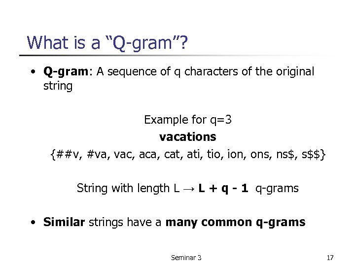
What is a “Q-gram”? • Q-gram: A sequence of q characters of the original string Example for q=3 vacations {##v, #va, vac, aca, cat, ati, tio, ion, ons, ns$, s$$} String with length L → L + q - 1 q-grams • Similar strings have a many common q-grams Seminar 3 17
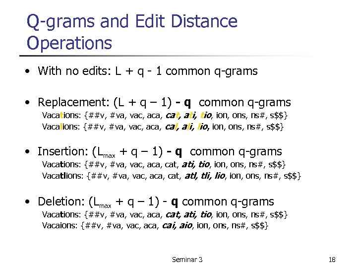
Q-grams and Edit Distance Operations • With no edits: L + q - 1 common q-grams • Replacement: (L + q – 1) - q common q-grams Vacations: {##v, #va, vac, aca, cat, ati, tio, ion, ons, ns#, s$$} Vacalions: {##v, #va, vac, aca, cal, ali, lio, ion, ons, ns#, s$$} • Insertion: (Lmax + q – 1) - q common q-grams Vacations: {##v, #va, vac, aca, cat, ati, tio, ion, ons, ns#, s$$} Vacatlions: {##v, #va, vac, aca, cat, atl, tli, lio, ion, ons, ns#, s$$} • Deletion: (Lmax + q – 1) - q common q-grams Vacations: {##v, #va, vac, aca, cat, ati, tio, ion, ons, ns#, s$$} Vacaions: {##v, #va, vac, aca, cai, aio, ion, ons, ns#, s$$} Seminar 3 18
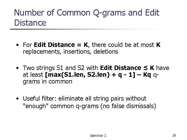
Number of Common Q-grams and Edit Distance • For Edit Distance = K, there could be at most K replacements, insertions, deletions • Two strings S 1 and S 2 with Edit Distance ≤ K have at least [max(S 1. len, S 2. len) + q - 1] – Kq qgrams in common • Useful filter: eliminate all string pairs without "enough" common q-grams (no false dismissals) Seminar 3 19
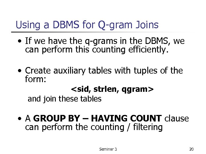
Using a DBMS for Q-gram Joins • If we have the q-grams in the DBMS, we can perform this counting efficiently. • Create auxiliary tables with tuples of the form: <sid, strlen, qgram> and join these tables • A GROUP BY – HAVING COUNT clause can perform the counting / filtering Seminar 3 20
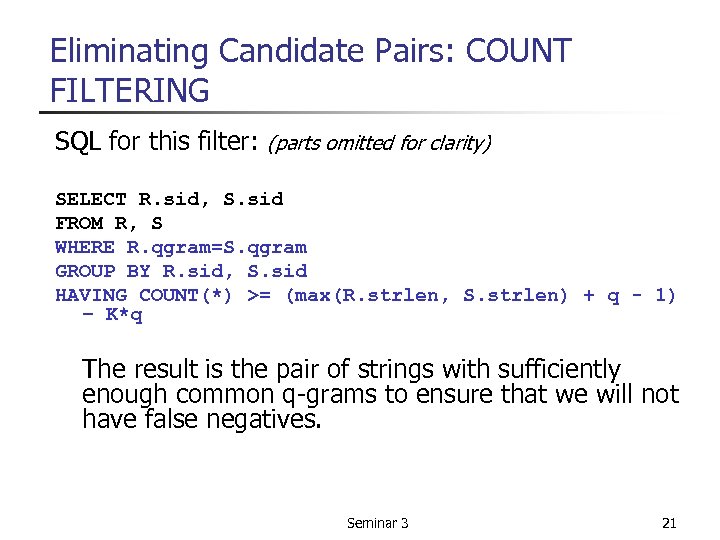
Eliminating Candidate Pairs: COUNT FILTERING SQL for this filter: (parts omitted for clarity) SELECT R. sid, S. sid FROM R, S WHERE R. qgram=S. qgram GROUP BY R. sid, S. sid HAVING COUNT(*) >= (max(R. strlen, S. strlen) + q - 1) – K*q The result is the pair of strings with sufficiently enough common q-grams to ensure that we will not have false negatives. Seminar 3 21
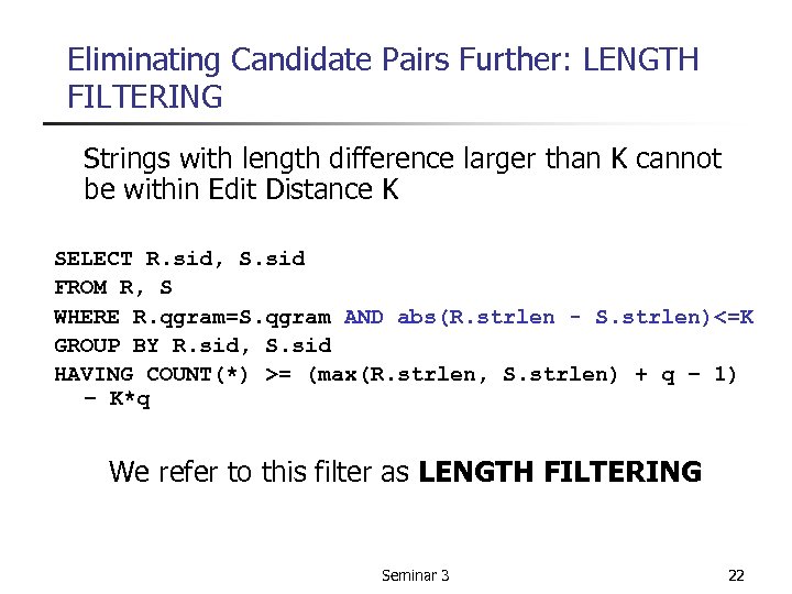
Eliminating Candidate Pairs Further: LENGTH FILTERING Strings with length difference larger than K cannot be within Edit Distance K SELECT R. sid, S. sid FROM R, S WHERE R. qgram=S. qgram AND abs(R. strlen - S. strlen)<=K GROUP BY R. sid, S. sid HAVING COUNT(*) >= (max(R. strlen, S. strlen) + q – 1) – K*q We refer to this filter as LENGTH FILTERING Seminar 3 22
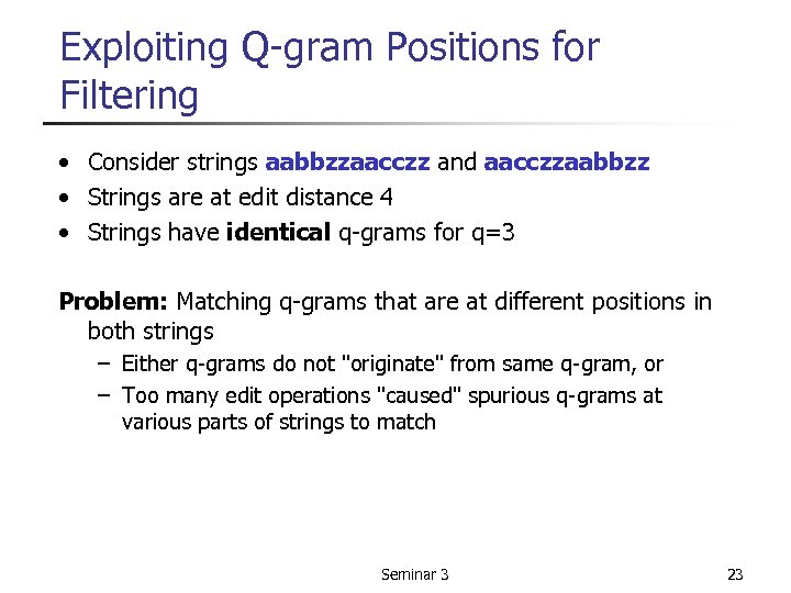
Exploiting Q-gram Positions for Filtering • Consider strings aabbzzaacczz and aacczzaabbzz • Strings are at edit distance 4 • Strings have identical q-grams for q=3 Problem: Matching q-grams that are at different positions in both strings – Either q-grams do not "originate" from same q-gram, or – Too many edit operations "caused" spurious q-grams at various parts of strings to match Seminar 3 23
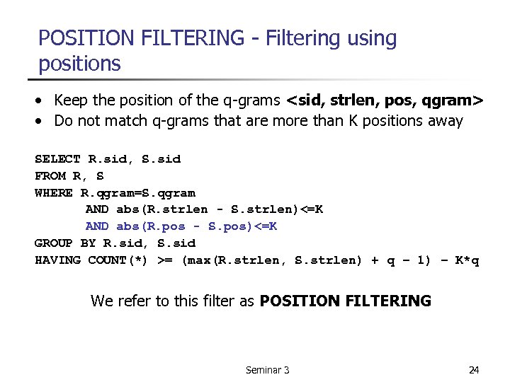
POSITION FILTERING - Filtering using positions • Keep the position of the q-grams <sid, strlen, pos, qgram> • Do not match q-grams that are more than K positions away SELECT R. sid, S. sid FROM R, S WHERE R. qgram=S. qgram AND abs(R. strlen - S. strlen)<=K AND abs(R. pos - S. pos)<=K GROUP BY R. sid, S. sid HAVING COUNT(*) >= (max(R. strlen, S. strlen) + q – 1) – K*q We refer to this filter as POSITION FILTERING Seminar 3 24
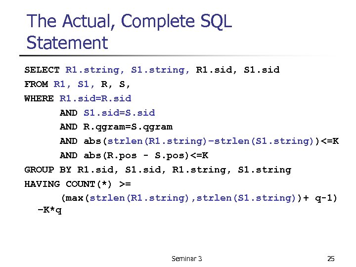
The Actual, Complete SQL Statement SELECT R 1. string, S 1. string, R 1. sid, S 1. sid FROM R 1, S 1, R, S, WHERE R 1. sid=R. sid AND S 1. sid=S. sid AND R. qgram=S. qgram AND abs(strlen(R 1. string)–strlen(S 1. string))<=K AND abs(R. pos - S. pos)<=K GROUP BY R 1. sid, S 1. sid, R 1. string, S 1. string HAVING COUNT(*) >= (max(strlen(R 1. string), strlen(S 1. string))+ q-1) –K*q Seminar 3 25
Summary of 1 st paper • Introduced a technique for mapping approximate string joins into a “vanilla” SQL expression • Our technique does not require modifying the underlying RDBMS Seminar 3 26
Outline • Supporting string-similarity joins using RDBMS • Using mapping techniques • Interactive deduplication Seminar 3 27
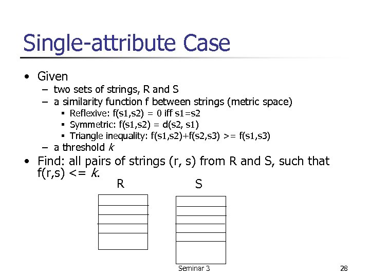
Single-attribute Case • Given – two sets of strings, R and S – a similarity function f between strings (metric space) § Reflexive: f(s 1, s 2) = 0 iff s 1=s 2 § Symmetric: f(s 1, s 2) = d(s 2, s 1) § Triangle inequality: f(s 1, s 2)+f(s 2, s 3) >= f(s 1, s 3) – a threshold k • Find: all pairs of strings (r, s) from R and S, such that f(r, s) <= k. R S Seminar 3 28
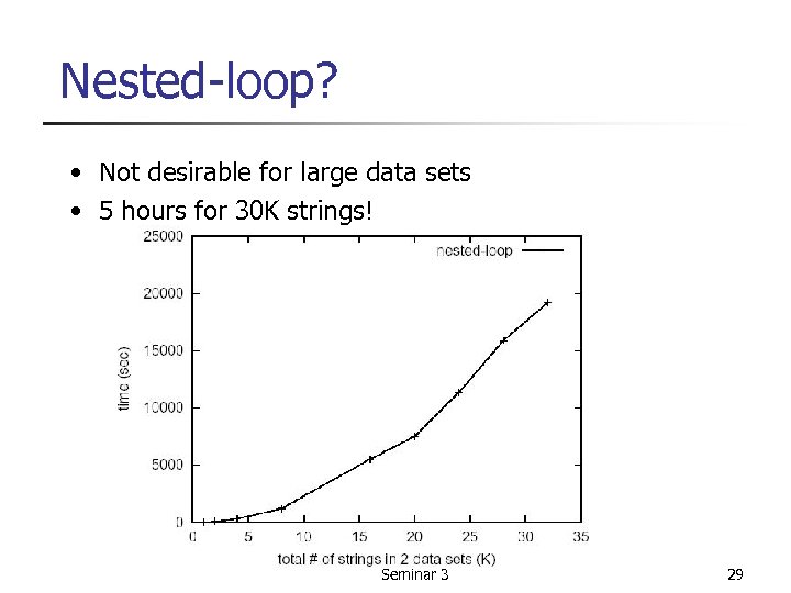
Nested-loop? • Not desirable for large data sets • 5 hours for 30 K strings! Seminar 3 29
Our 2 -step approach • Step 1: map strings (in a metric space) to objects in a Euclidean space • Step 2: do a similarity join in the Euclidean space Seminar 3 30
Advantages • Applicable to many metric similarity functions – Use edit distance as an example – Other similarity functions also tried, e. g. , qgram-based similarity • Open to existing algorithms – Mapping techniques – Join techniques Seminar 3 31
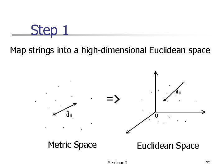
Step 1 Map strings into a high-dimensional Euclidean space Metric Space Euclidean Space Seminar 3 32
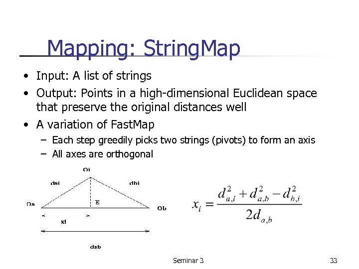
Mapping: String. Map • Input: A list of strings • Output: Points in a high-dimensional Euclidean space that preserve the original distances well • A variation of Fast. Map – Each step greedily picks two strings (pivots) to form an axis – All axes are orthogonal Seminar 3 33
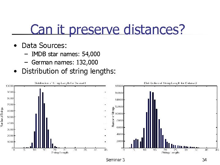
Can it preserve distances? • Data Sources: – IMDB star names: 54, 000 – German names: 132, 000 • Distribution of string lengths: Seminar 3 34
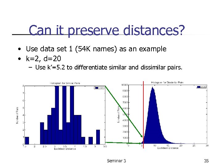
Can it preserve distances? • Use data set 1 (54 K names) as an example • k=2, d=20 – Use k’=5. 2 to differentiate similar and dissimilar pairs. Seminar 3 35
Choose Dimensionality d Increase d? • Good : – better to differentiate similar pairs from dissimilar ones. • Bad : – Step 1: Efficiency ↓ – Step 2: “curse of dimensionality” Seminar 3 36
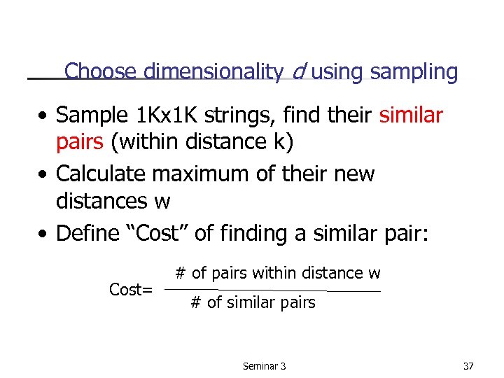
Choose dimensionality d using sampling • Sample 1 Kx 1 K strings, find their similar pairs (within distance k) • Calculate maximum of their new distances w • Define “Cost” of finding a similar pair: Cost= # of pairs within distance w # of similar pairs Seminar 3 37
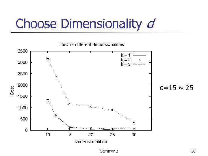
Choose Dimensionality d d=15 ~ 25 Seminar 3 38
Choose new threshold k’ • Closely related to the mapping property • Ideally, if ed(r, s) <= k, the Euclidean distance between two corresponding points <= k’. • Choose k’ using sampling – Sample 1 Kx 1 K strings, find similar pairs – Calculate their maximum new distance as k’ – repeat multiple times, choose their maximum Seminar 3 39
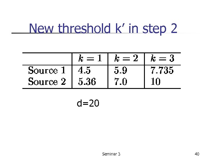
New threshold k’ in step 2 d=20 Seminar 3 40
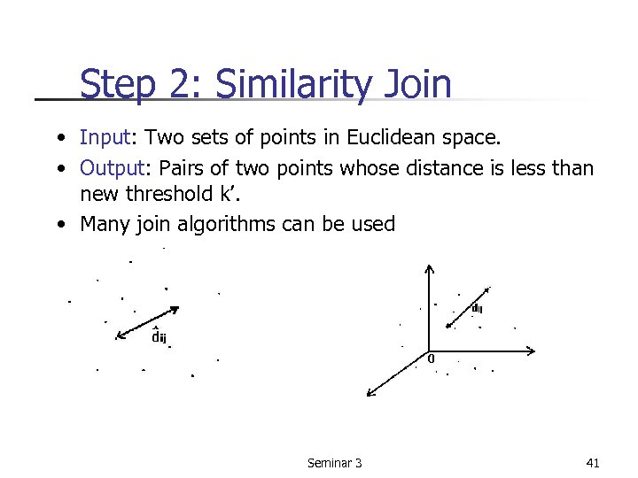
Step 2: Similarity Join • Input: Two sets of points in Euclidean space. • Output: Pairs of two points whose distance is less than new threshold k’. • Many join algorithms can be used Seminar 3 41
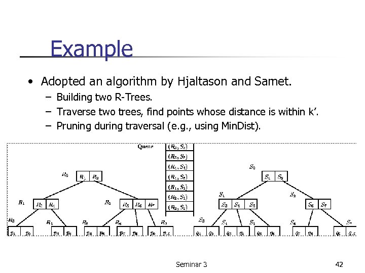
Example • Adopted an algorithm by Hjaltason and Samet. – Building two R-Trees. – Traverse two trees, find points whose distance is within k’. – Pruning during traversal (e. g. , using Min. Dist). Seminar 3 42
Final processing • Among the pairs produced from the similarity-join step, check their edit distance. • Return those pairs satisfying the threshold k Seminar 3 43
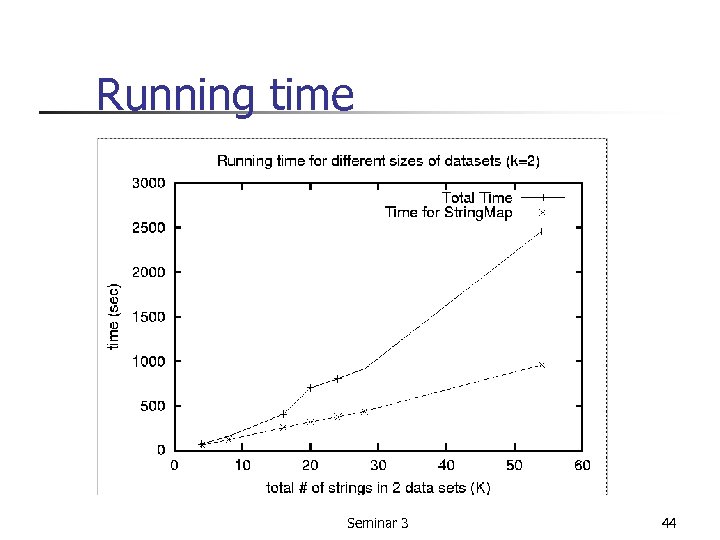
Running time Seminar 3 44
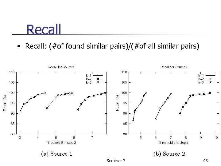
Recall • Recall: (#of found similar pairs)/(#of all similar pairs) Seminar 3 45
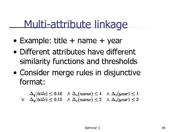
Multi-attribute linkage • Example: title + name + year • Different attributes have different similarity functions and thresholds • Consider merge rules in disjunctive format: Seminar 3 46
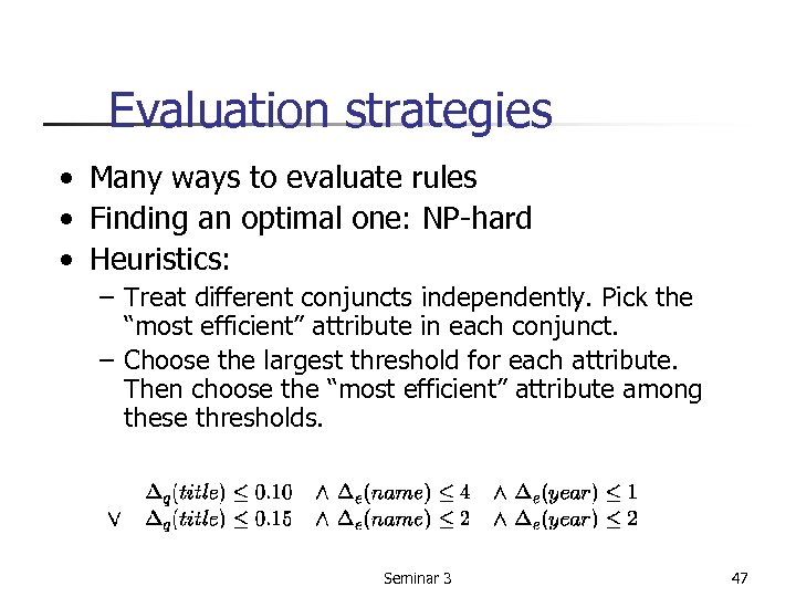
Evaluation strategies • Many ways to evaluate rules • Finding an optimal one: NP-hard • Heuristics: – Treat different conjuncts independently. Pick the “most efficient” attribute in each conjunct. – Choose the largest threshold for each attribute. Then choose the “most efficient” attribute among these thresholds. Seminar 3 47
Summary of 2 nd paper • A novel two-step approach to record linkage. • Many existing mapping and join algorithms can be adopted • Applicable to many distance metrics. • Time and space efficient. • Multi-attribute case studied Seminar 3 48
Outline • Supporting string-similarity joins using RDBMS • Using mapping techniques • Interactive deduplication Seminar 3 49
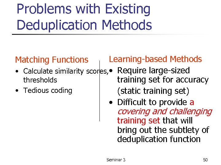
Problems with Existing Deduplication Methods Learning-based Methods • Calculate similarity scores, • Require large-sized thresholds training set for accuracy • Tedious coding (static training set) • Difficult to provide a Matching Functions covering and challenging training set that will bring out the subtlety of deduplication function Seminar 3 50
New Approach • Relegate the task of finding the deduplication function to a machine learning algorithm • Design goal: § Less training instances § Interactive response § Fast convergence § High accuracy Design an interactive deduplication system called ALIAS: Active Learning led Interactive Alias Suppression 51
ALIAS SYSTEM • A learned-based method • Exploit existing similarity functions • Use Active Learning - an active learner actively picks unlabeled instances with the most information gain in the training set • Produce a deduplication function that can identify duplicates 52
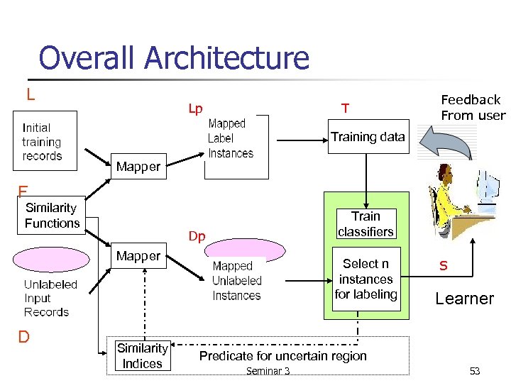
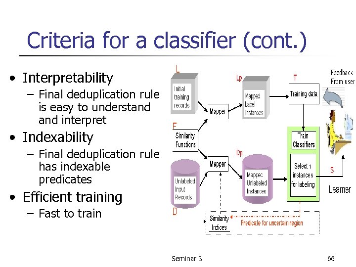
Overall Architecture L Lp T Feedback From user Training data Mapper F Similarity Functions Train classifiers Dp Mapper D Similarity Indices Select n instances for labeling S Learner Predicate for uncertain region Seminar 3 53
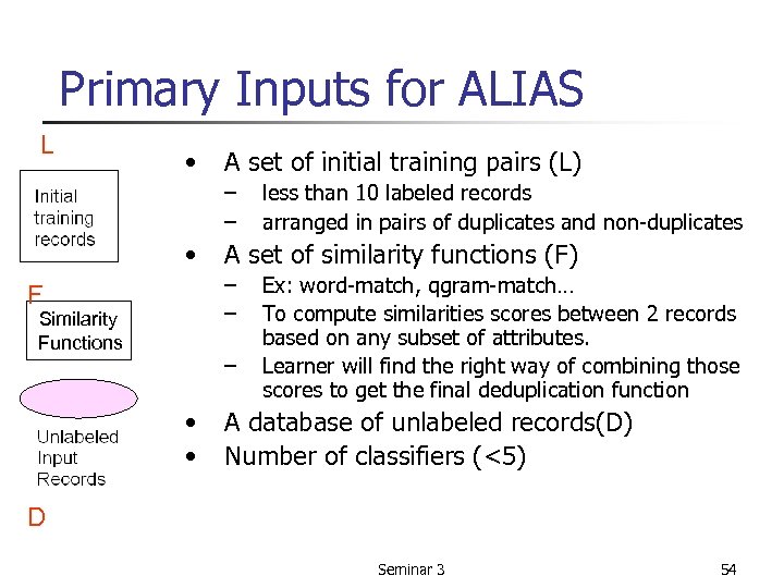
Primary Inputs for ALIAS L • A set of initial training pairs (L) – – • A set of similarity functions (F) – – F Similarity Functions – • • less than 10 labeled records arranged in pairs of duplicates and non-duplicates Ex: word-match, qgram-match… To compute similarities scores between 2 records based on any subset of attributes. Learner will find the right way of combining those scores to get the final deduplication function A database of unlabeled records(D) Number of classifiers (<5) D Seminar 3 54
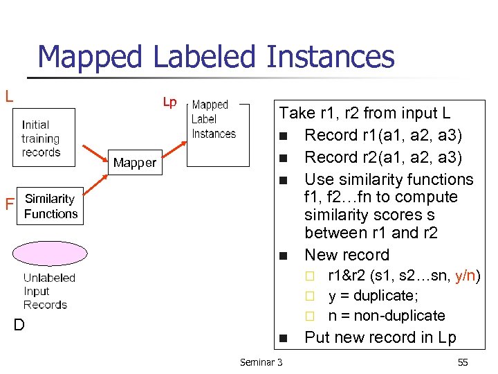
Mapped Labeled Instances L Lp Mapper F Similarity Functions Take r 1, r 2 from input L n Record r 1(a 1, a 2, a 3) n Record r 2(a 1, a 2, a 3) n Use similarity functions f 1, f 2…fn to compute similarity scores s between r 1 and r 2 n New record r 1&r 2 (s 1, s 2…sn, y/n) ¨ y = duplicate; ¨ n = non-duplicate ¨ D n Seminar 3 Put new record in Lp 55
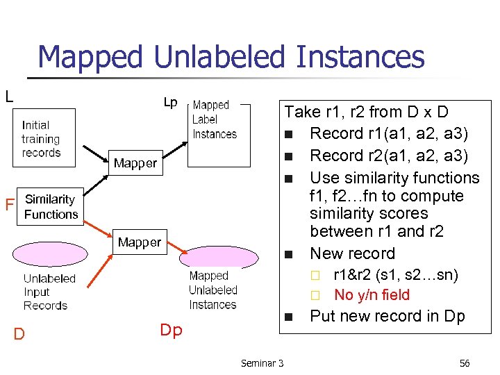
Mapped Unlabeled Instances L Lp Take r 1, r 2 from D x D n Record r 1(a 1, a 2, a 3) n Record r 2(a 1, a 2, a 3) n Use similarity functions f 1, f 2…fn to compute similarity scores between r 1 and r 2 n New record Mapper F Similarity Functions Mapper r 1&r 2 (s 1, s 2…sn) ¨ No y/n field ¨ D n Dp Seminar 3 Put new record in Dp 56
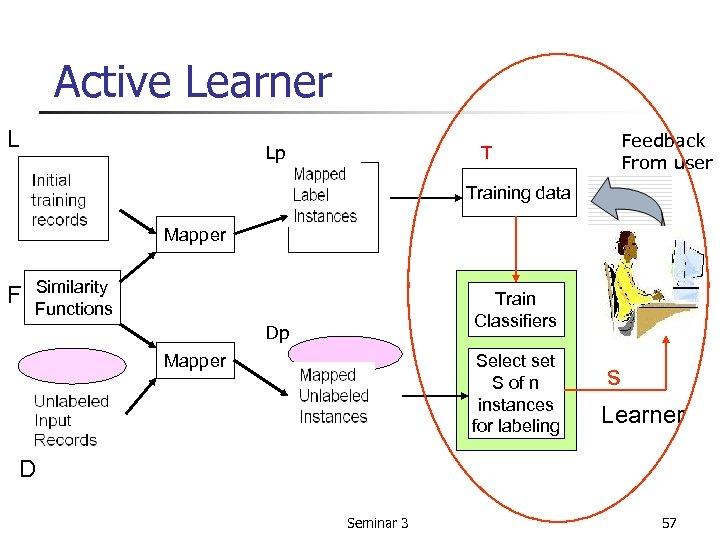
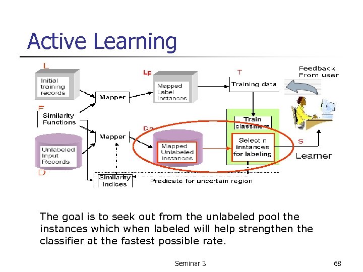
Active Learner L Lp T Feedback From user Training data Mapper F Similarity Functions Train Classifiers Dp Mapper Select set S of n instances for labeling s Learner D Seminar 3 57
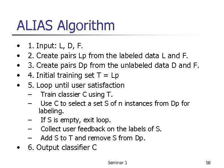
ALIAS Algorithm • • • 1. 2. 3. 4. 5. – – – • Input: L, D, F. Create pairs Lp from the labeled data L and F. Create pairs Dp from the unlabeled data D and F. Initial training set T = Lp Loop until user satisfaction Train classier C using T. Use C to select a set S of n instances from Dp for labeling. If S is empty, exit loop. Collect user feedback on the labels of S. Add S to T and remove S from Dp. 6. Output classifier C Seminar 3 58
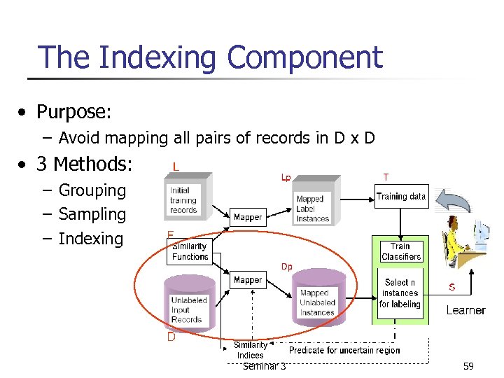
The Indexing Component • Purpose: – Avoid mapping all pairs of records in D x D • 3 Methods: – Grouping – Sampling – Indexing Seminar 3 59
The Indexing Component • Grouping – Example: group records in D according to the field year of publication – Mapped pairs are formed only within records of a group. • Sampling – Sample in units of a group instead of individual records. Seminar 3 60
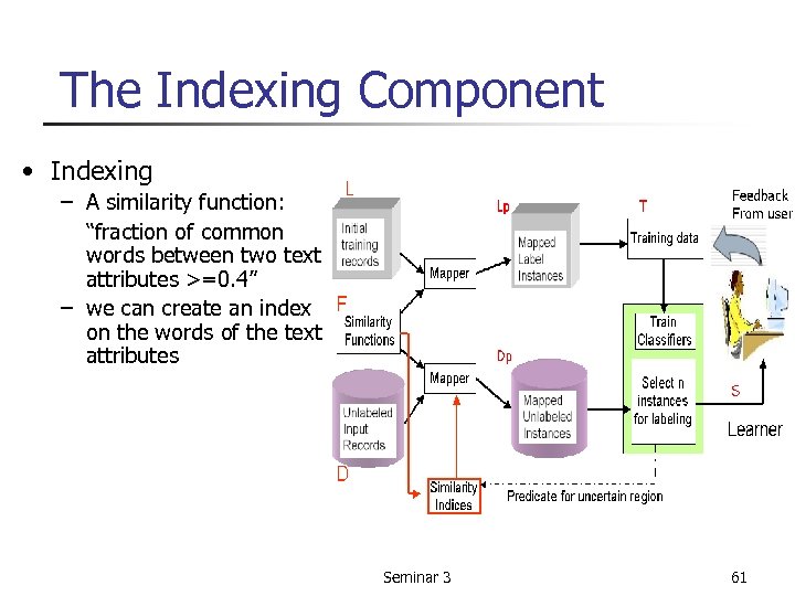
The Indexing Component • Indexing – A similarity function: “fraction of common words between two text attributes >=0. 4” – we can create an index on the words of the text attributes Seminar 3 61
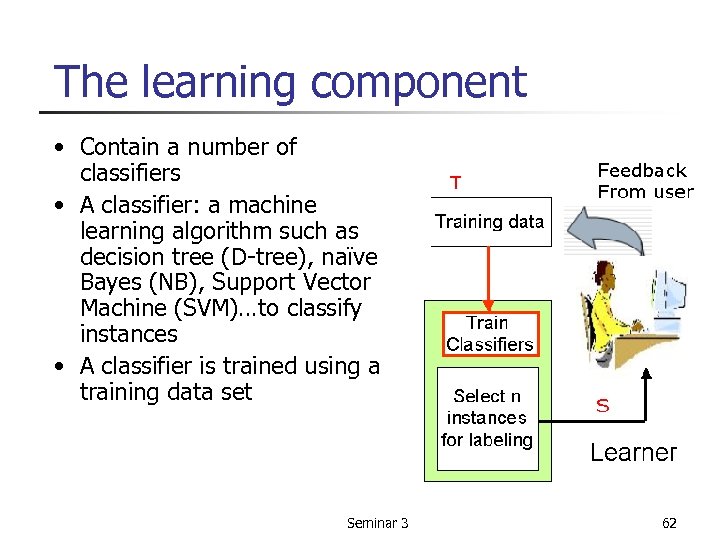
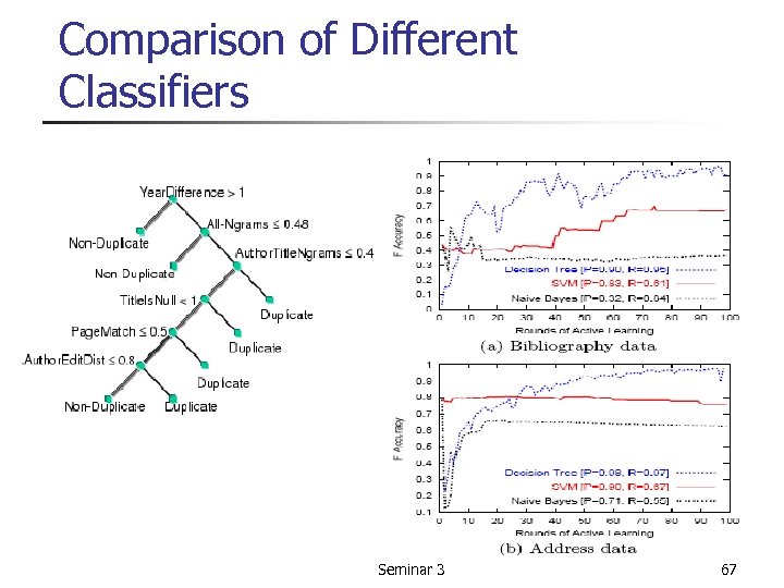
The learning component • Contain a number of classifiers • A classifier: a machine learning algorithm such as decision tree (D-tree), naïve Bayes (NB), Support Vector Machine (SVM)…to classify instances • A classifier is trained using a training data set Seminar 3 62
Criteria for a classifier • • Accuracy Interpretability Indexability Efficient training Seminar 3 63
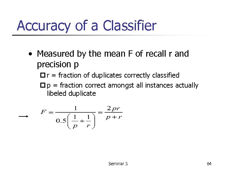
Accuracy of a Classifier • Measured by the mean F of recall r and precision p p r = fraction of duplicates correctly classified p p = fraction correct amongst all instances actually libeled duplicate Seminar 3 64
Accuracy (cont. ) n Example A case with 1% duplicates; a classifier labels all pairs as non-duplicates recall r = 0 mean F = 0 accuracy = 0% ¨ A case with 1% duplicates; a classifier identifies all duplicates correctly but misclassifies 1% non-duplicates recall r = 1, p = 0. 5 F = 0. 667 accuracy = 66. 7% ¨ If we don’t use r and p, then they both have 99% accuracy! Seminar 3 65
Criteria for a classifier (cont. ) • Interpretability – Final deduplication rule is easy to understand interpret • Indexability – Final deduplication rule has indexable predicates • Efficient training – Fast to train Seminar 3 66
Comparison of Different Classifiers Seminar 3 67
Active Learning The goal is to seek out from the unlabeled pool the instances which when labeled will help strengthen the classifier at the fastest possible rate. Seminar 3 68
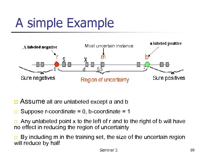
A simple Example Most uncertain instance o Assume all are unlabeled except a and b o Suppose r-coordinate = 0, b-coordinate = 1 Any unlabeled point x to the left of r and to the right of b will have no effect in reducing the region of uncertainty o By including m in the training set, the size of the uncertain region will reduce by half o Seminar 3 69
How to select an unlabeled instance • Uncertainty – The instance about which the learner was most unsure was also the instance for which the expected reduction in confusion was the largest – Uncertainty score § the disagreement among the predictions the instance get from a committee of N classifiers § A sure duplicate or non-duplicate would get the same prediction from all members • Representativeness – An uncertain instance representing a larger number of unlabeled instances has greater impact to the classifier Seminar 3 70
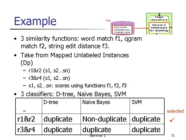
Example • 3 similarity functions: word match f 1, qgram match f 2, string edit distance f 3. • Take from Mapped Unlabeled Instances (Dp) – r 1&r 2 (s 1, s 2…sn) – r 3&r 4 (s 1, s 2…sn) – s 1, s 2…sn: scores using functions f 1, f 2, f 3 • 3 classifiers: D-tree, Naïve Bayes, SVM D-tree Naïve Bayes SVM – r 1&r 2 r 3&r 4 selected duplicate Non-duplicate Seminar 3 ü 71
How to Combine Uncertainty and Representativeness – Proposed two approaches – 1 st approach: weighted sum § Cluster the unlabeled instances § Estimate the density of points around it § The instances are scored using a weighted sum of its density and uncertainty value § n highest scoring instances selected – 2 nd approach: sampling Seminar 3 72
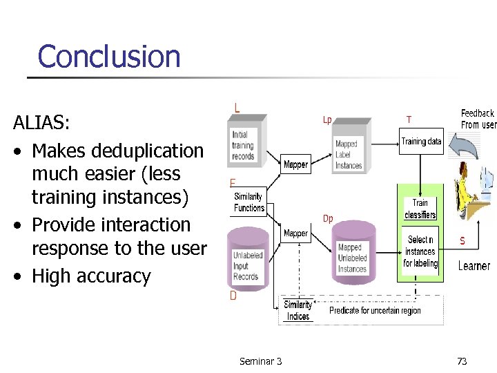
Conclusion ALIAS: • Makes deduplication much easier (less training instances) • Provide interaction response to the user • High accuracy Seminar 3 73
c9ac1616f1164496d9a05db1ea321b3e.ppt