a0a467c67c041debaf89495b39249416.ppt
- Количество слайдов: 164
 Search and Decoding in Speech Recognition N-Grams
 N-Grams u u u Problem of word prediction. Example: “I’d like to make a collect …” n Very likely words: u “call”, u “international call”, or u “phone call”, and NOT u “the”. The idea of word prediction is formalized with probabilistic models called N-grams. n N-grams – predict the next word from previous N-1 words. n Statistical models of word sequences are also called language models or LMs. Computing probability of the next word will turn out to be closely related to computing the probability of a sequence of words. Example: n “… all of a sudden I notice three guys standing on the sidewalk …”, vs. n “… on guys all I of notice sidewalk three a sudden standing the …” 3/19/2018 Veton Këpuska 2
 N-grams u Estimators like N-grams that assign a conditional probability to possible next words can be used to assign a joint probability to an entire sentence. u N-gram models are on of the most important tools in speech and language processing. u N-grams are essential in any tasks in which the words must be identified from ambiguous and noisy inputs. u Speech Recognition – the input speech sounds are very confusable and many words sound extremely similar. 3/19/2018 Veton Këpuska 3
 N-gram u Handwriting Recognition – probabilities of word sequences help in recognition. n Woody Allen in his movie “Take the Money and Run”, tries to rob a bank with a sloppily written hold-up note that the teller incorrectly reads as “I have a gub”. n Any speech and language processing system could avoid making this mistake by using the knowledge that the sequence “I have a gun” is far more probable than the non-word “I have a gub” or even “I have a gull”. 3/19/2018 Veton Këpuska 4
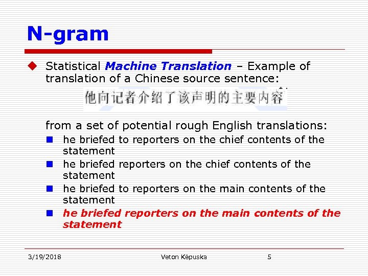 N-gram u Statistical Machine Translation – Example of translation of a Chinese source sentence: from a set of potential rough English translations: n he briefed to reporters on the chief contents of the statement n he briefed to reporters on the main contents of the statement n he briefed reporters on the main contents of the statement 3/19/2018 Veton Këpuska 5
 N-gram u An N-grammar might tell us that briefed reporters is more likely than briefed to reporters, and main contents is more likely than chief contents. u Spelling Corrections – need to find correct spelling errors like the following that accidentally result in real English words: n They are leaving in about fifteen minuets to go to her house. n The design an construction of the system will take more than a year. u Problem – real words thus dictionary search will not help. n Note: “in about fifteen minuets” is a much less probable sequence than “in about fifteen minutes” n Spell-checker can use a probability estimator both to detect these errors and to suggest higher-probability corrections. 3/19/2018 Veton Këpuska 6
 N-gram u Augmentative Communication – helping people who are unable to sue speech or sign language to communicate (Steven Hawking). n Using simple body movements to select words from a menu that are spoken by the system. n Word prediction can be used to suggest likely words for the menu. u Other areas: n Part of-speech tagging n Natural Language Generation, n Word Similarity, n Authorship identification n Sentiment Extraction n Predictive Text Input (Cell phones). 3/19/2018 Veton Këpuska 7
 Corpora & Counting Words u Probabilities are based on counting things. n Must decide what to count. n Counting things in natural language is based on a corpus (plural corpora) – an on-line collection of text or speech. n Popular corpora “Brown” and “Switchboard”. u Brown corpus is a 1 million word collection of samples from 500 written texts from different genres (newspaper, novels, non-fiction, academic, etc. ) assembled at Brown university 1963 -1964. n Example sentence from Brown corpus: u He stepped out into the hall, was delighted to encounter a water brother. u 13 words if don’t’ count punctuation-marks as words – 15 if we count punctuation. u Treatment of “, ” and “. ” depends on the task. u Punctuation marks are critical for identifying boundaries (, . ; ) of things and for identifying some aspects of meaning (? ! ”) u For some tasks (part-of-speech tagging or parsing or sometimes speech synthesis) punctuation are treated as being separate words. 3/19/2018 Veton Këpuska 8
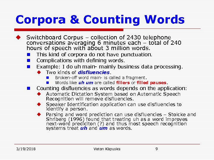 Corpora & Counting Words u Switchboard Corpus – collection of 2430 telephone conversations averaging 6 minutes each – total of 240 hours of speech with about 3 million words. n n n This kind of corpora do not have punctuation. Complications with defining words. Example: I do uh main- mainly business data processing. u Two kinds of disfluencies. n n n Broken-off word main- is called a fragment. Words like uh um are called fillers or filled pauses. Counting disfluencies as words depends on the application: u Automatic Dictation System based on Automatic Speech Recognition will remove disfluencies. u Speaker Identification application can use disfluencies to identify a person. u Parsing and word prediction can use disfluencies – Stolcke and Shriberg (1996) found that treating uh as a word improves next-word prediciton (? ) and thus most speech recognition systems treat uh and um as words. 3/19/2018 Veton Këpuska 9
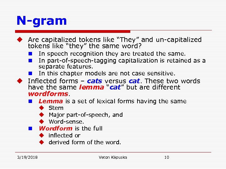 N-gram u Are capitalized tokens like “They” and un-capitalized tokens like “they” the same word? n n n In speech recognition they are treated the same. In part-of-speech-tagging capitalization is retained as a separate features. In this chapter models are not case sensitive. u Inflected forms – cats versus cat. These two words have the same lemma “cat” but are different wordforms. n n 3/19/2018 Lemma is a set of lexical forms having the same u Stem u Major part-of-speech, and u Word-sense. Wordform is the full u inflected or u derived form of the word. Veton Këpuska 10
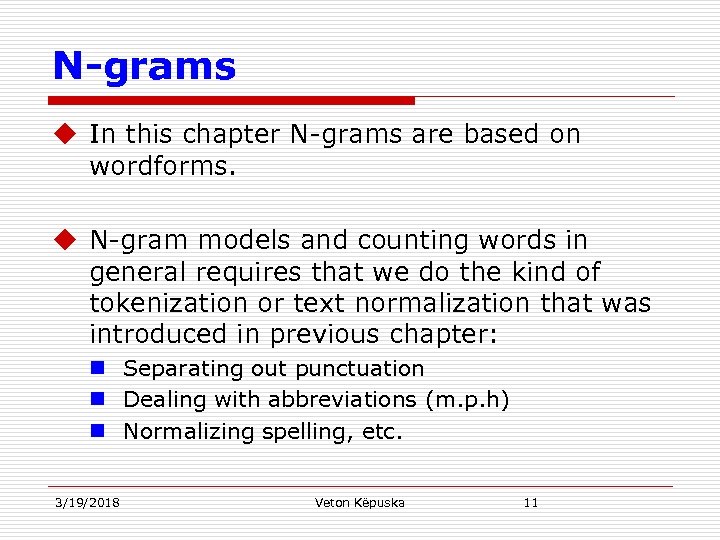 N-grams u In this chapter N-grams are based on wordforms. u N-gram models and counting words in general requires that we do the kind of tokenization or text normalization that was introduced in previous chapter: n Separating out punctuation n Dealing with abbreviations (m. p. h) n Normalizing spelling, etc. 3/19/2018 Veton Këpuska 11
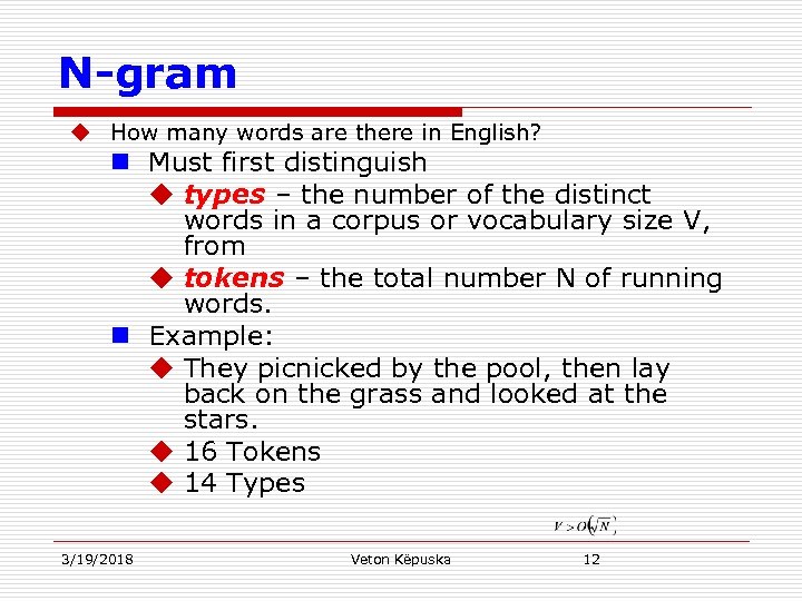 N-gram u How many words are there in English? n Must first distinguish u types – the number of the distinct words in a corpus or vocabulary size V, from u tokens – the total number N of running words. n Example: u They picnicked by the pool, then lay back on the grass and looked at the stars. u 16 Tokens u 14 Types 3/19/2018 Veton Këpuska 12
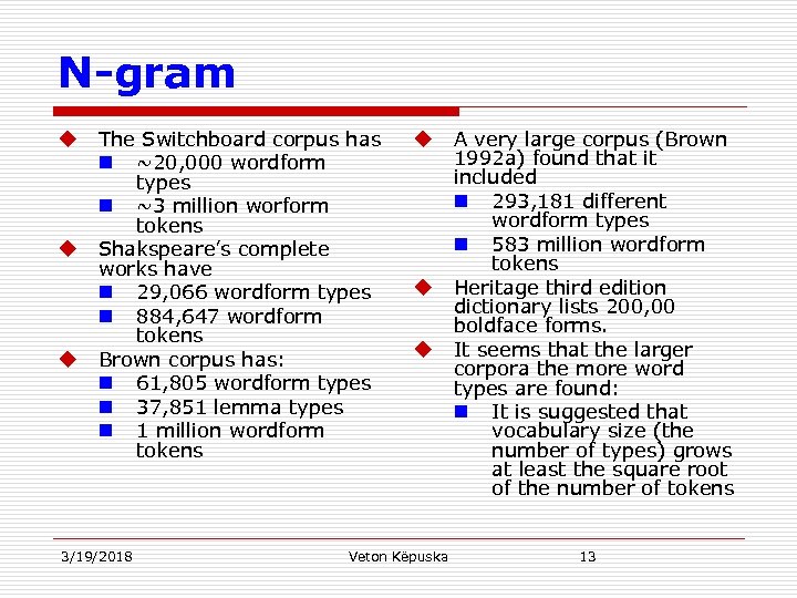 N-gram u u u The Switchboard corpus has n ~20, 000 wordform types n ~3 million worform tokens Shakspeare’s complete works have n 29, 066 wordform types n 884, 647 wordform tokens Brown corpus has: n 61, 805 wordform types n 37, 851 lemma types n 1 million wordform tokens 3/19/2018 u u u Veton Këpuska A very large corpus (Brown 1992 a) found that it included n 293, 181 different wordform types n 583 million wordform tokens Heritage third edition dictionary lists 200, 00 boldface forms. It seems that the larger corpora the more word types are found: n It is suggested that vocabulary size (the number of types) grows at least the square root of the number of tokens 13
 Brief Introduction to Probability Discrete Probability
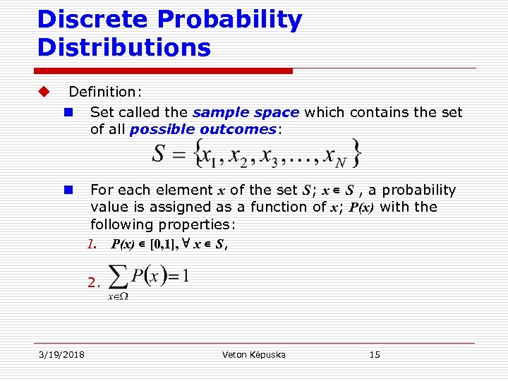 Discrete Probability Distributions u Definition: n Set called the sample space which contains the set of all possible outcomes: n For each element x of the set S; x ∊ S , a probability value is assigned as a function of x; P(x) with the following properties: 1. P(x) ∊ [0, 1], ∀ x ∊ S, 2. 3/19/2018 Veton Këpuska 15
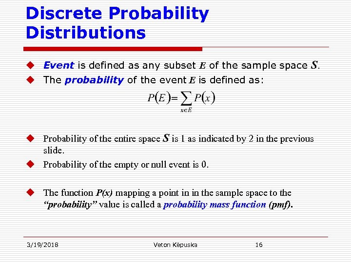 Discrete Probability Distributions u Event is defined as any subset E of the sample space S. u The probability of the event E is defined as: u Probability of the entire space S is 1 as indicated by 2 in the previous slide. u Probability of the empty or null event is 0. u The function P(x) mapping a point in in the sample space to the “probability” value is called a probability mass function (pmf). 3/19/2018 Veton Këpuska 16
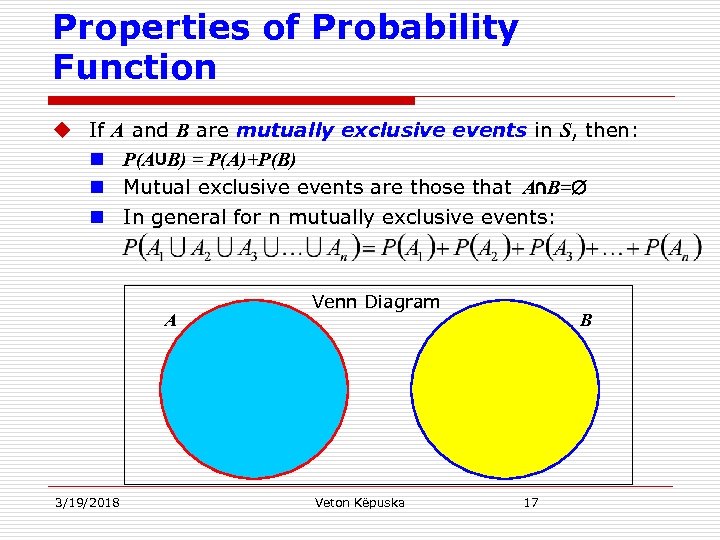 Properties of Probability Function u If n n n A and B are mutually exclusive events in S, then: P(A∪B) = P(A)+P(B) Mutual exclusive events are those that A∩B=∅ In general for n mutually exclusive events: A 3/19/2018 Venn Diagram Veton Këpuska B 17
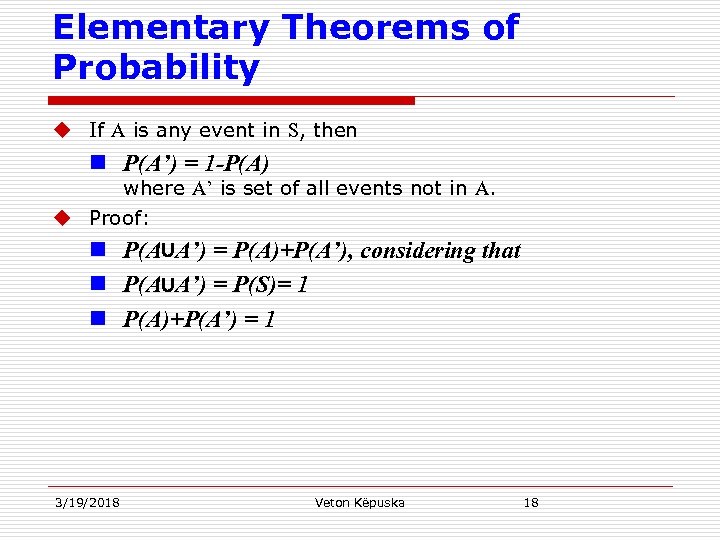 Elementary Theorems of Probability u If A is any event in S, then n P(A’) = 1 -P(A) where A’ is set of all events not in A. u Proof: n P(A∪A’) = P(A)+P(A’), considering that n P(A∪A’) = P(S)= 1 n P(A)+P(A’) = 1 3/19/2018 Veton Këpuska 18
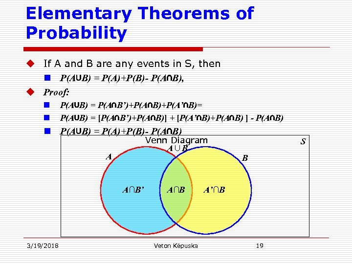 Elementary Theorems of Probability u If A and B are any events in S, then n P(A∪B) = P(A)+P(B)- P(A∩B), u Proof: n n P(A∪B) = P(A∩B’)+P(A∩B)+P(A’∩B)= P(A∪B) = [P(A∩B’)+P(A∩B)] + [P(A’∩B)+P(A∩B) ] - P(A∩B) n P(A∪B) = P(A)+P(B)- P(A∩B) Venn Diagram A∪B A A∩B’ 3/19/2018 A∩B Veton Këpuska S B A’∩B 19
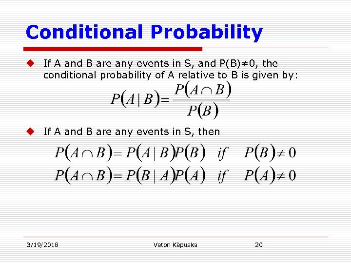 Conditional Probability u If A and B are any events in S, and P(B)≠ 0, the conditional probability of A relative to B is given by: u If A and B are any events in S, then 3/19/2018 Veton Këpuska 20
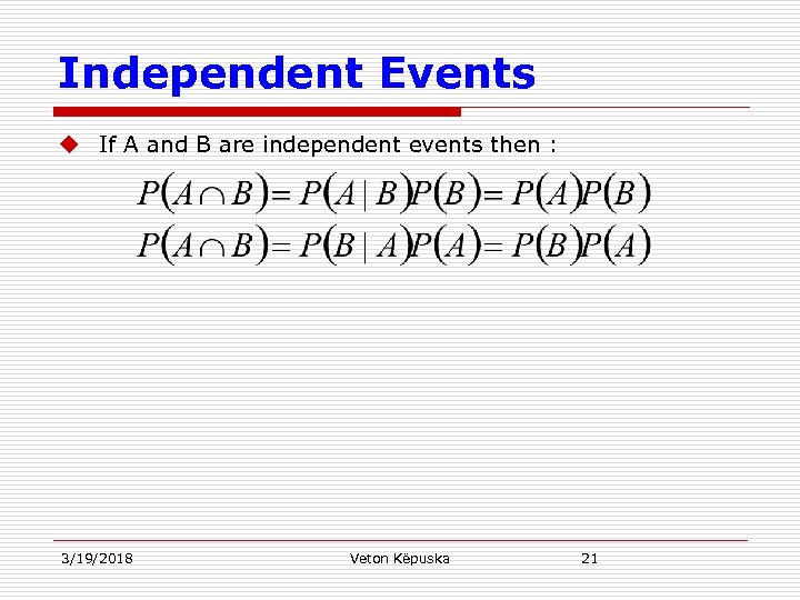 Independent Events u If A and B are independent events then : 3/19/2018 Veton Këpuska 21
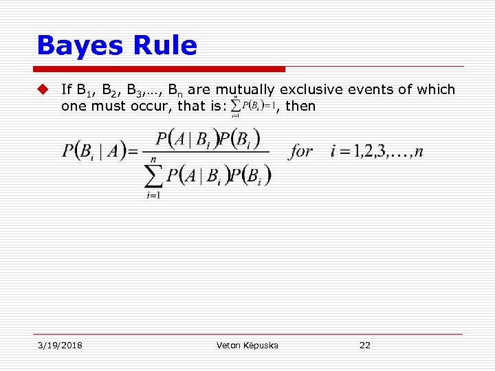 Bayes Rule u If B 1, B 2, B 3, …, Bn are mutually exclusive events of which one must occur, that is: , then 3/19/2018 Veton Këpuska 22
 End of Brief Introduction to Probability End
 Simple N-grams
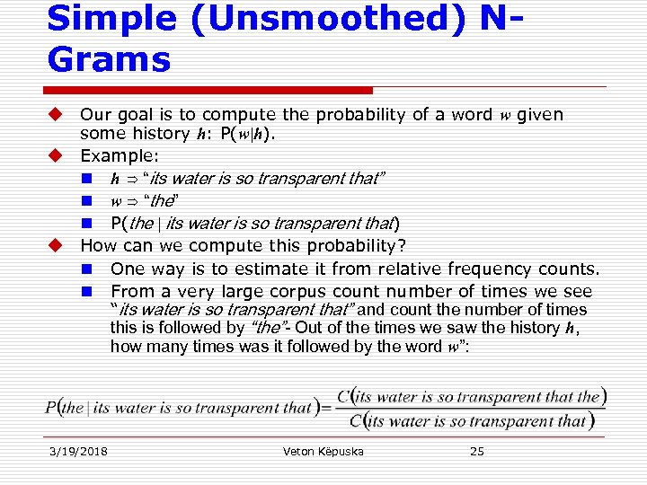 Simple (Unsmoothed) NGrams u Our goal is to compute the probability of a word w given some history h: P(w|h). u Example: n h ⇒ “its water is so transparent that” n w ⇒ “the” n P(the | its water is so transparent that) u How can we compute this probability? n One way is to estimate it from relative frequency counts. n From a very large corpus count number of times we see “its water is so transparent that” and count the number of times this is followed by “the”- Out of the times we saw the history h, how many times was it followed by the word w”: 3/19/2018 Veton Këpuska 25
 Estimating Probabilities u Estimating probabilities form counts works fine in many cases, it turns out that even the www is not big enough to give us good estimates in most cases. n Language is creative: 1. new sentences are created all the time. 2. It is not possible to count entire sentences. 3/19/2018 Veton Këpuska 26
 Estimating Probabilities u Joint Probabilities – probability of an entire sequence of words like “its water is so transparent”: n Out of all possible sequences of 5 words how many of them are “its water is so transparent” n Must count of all occurrences of “its water is so transparent” and divide by the sum of counts of all possible 5 word sequences. u It seems a lot of work for a simple computation of estimates. 3/19/2018 Veton Këpuska 27
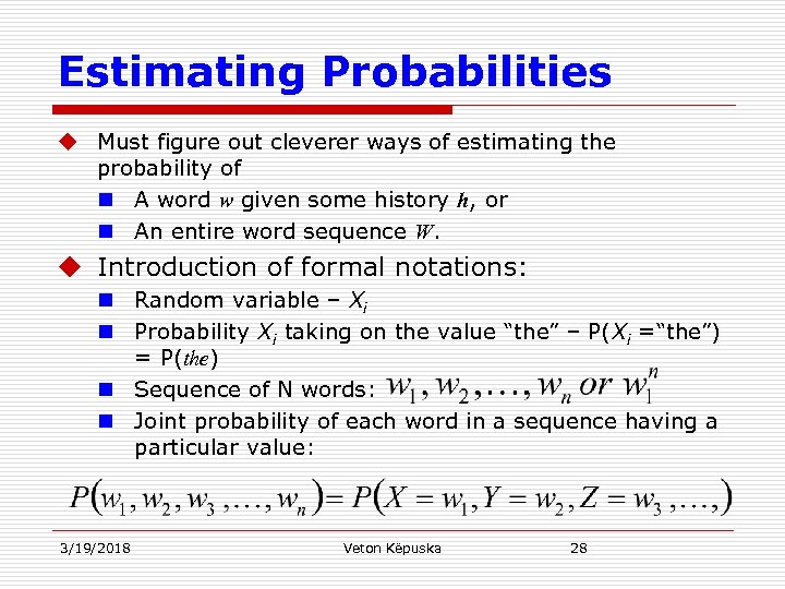 Estimating Probabilities u Must figure out cleverer ways of estimating the probability of n A word w given some history h, or n An entire word sequence W. u Introduction of formal notations: n Random variable – Xi n Probability Xi taking on the value “the” – P(Xi =“the”) = P(the) n Sequence of N words: n Joint probability of each word in a sequence having a particular value: 3/19/2018 Veton Këpuska 28
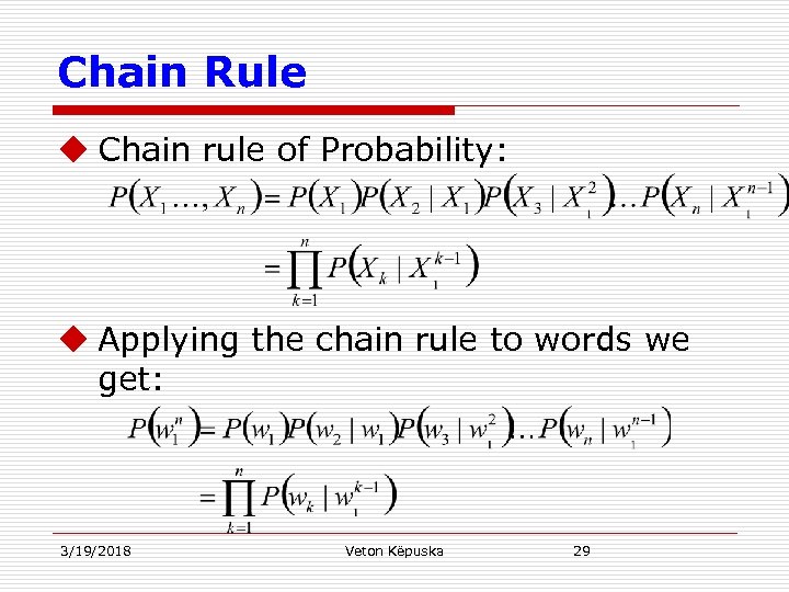 Chain Rule u Chain rule of Probability: u Applying the chain rule to words we get: 3/19/2018 Veton Këpuska 29
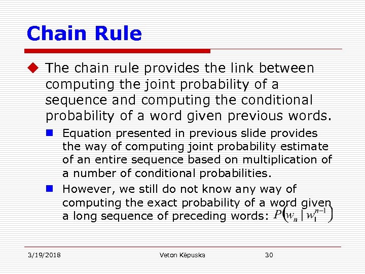 Chain Rule u The chain rule provides the link between computing the joint probability of a sequence and computing the conditional probability of a word given previous words. n Equation presented in previous slide provides the way of computing joint probability estimate of an entire sequence based on multiplication of a number of conditional probabilities. n However, we still do not know any way of computing the exact probability of a word given a long sequence of preceding words: 3/19/2018 Veton Këpuska 30
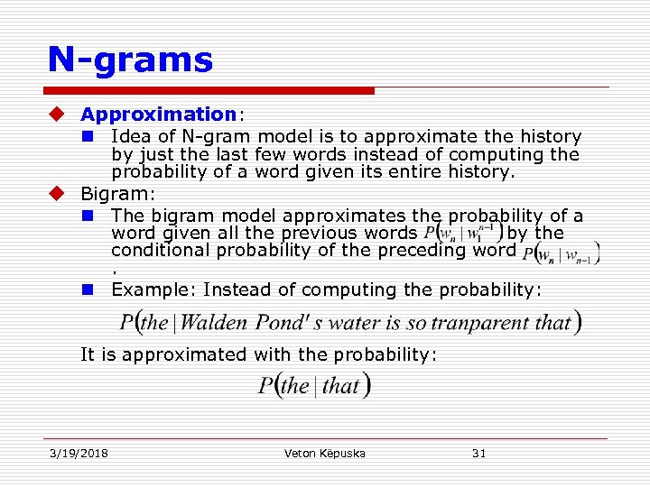 N-grams u Approximation: n Idea of N-gram model is to approximate the history by just the last few words instead of computing the probability of a word given its entire history. u Bigram: n The bigram model approximates the probability of a word given all the previous words by the conditional probability of the preceding word. n Example: Instead of computing the probability: It is approximated with the probability: 3/19/2018 Veton Këpuska 31
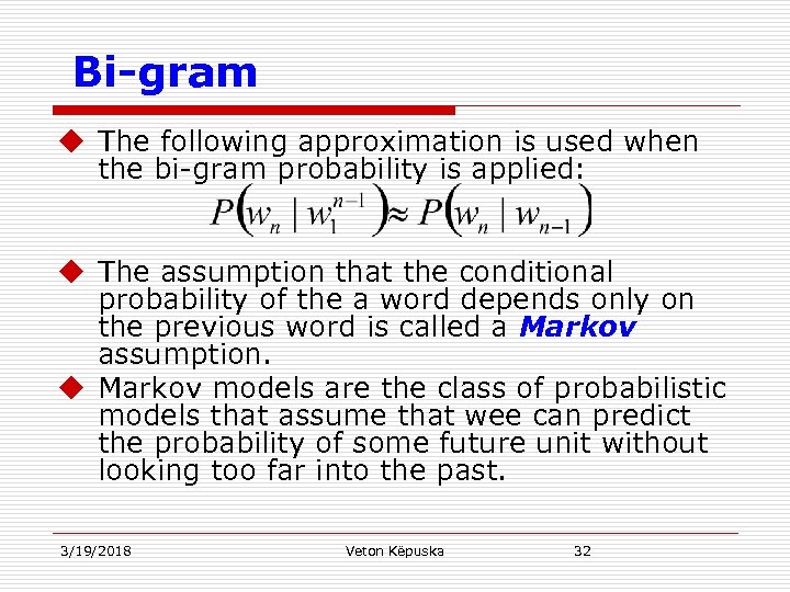 Bi-gram u The following approximation is used when the bi-gram probability is applied: u The assumption that the conditional probability of the a word depends only on the previous word is called a Markov assumption. u Markov models are the class of probabilistic models that assume that wee can predict the probability of some future unit without looking too far into the past. 3/19/2018 Veton Këpuska 32
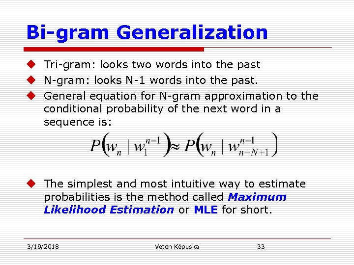 Bi-gram Generalization u Tri-gram: looks two words into the past u N-gram: looks N-1 words into the past. u General equation for N-gram approximation to the conditional probability of the next word in a sequence is: u The simplest and most intuitive way to estimate probabilities is the method called Maximum Likelihood Estimation or MLE for short. 3/19/2018 Veton Këpuska 33
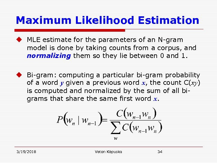 Maximum Likelihood Estimation u MLE estimate for the parameters of an N-gram model is done by taking counts from a corpus, and normalizing them so they lie between 0 and 1. u Bi-gram: computing a particular bi-gram probability of a word y given a previous word x, the count C(xy) is computed and normalized by the sum of all bigrams that share the same first word x. 3/19/2018 Veton Këpuska 34
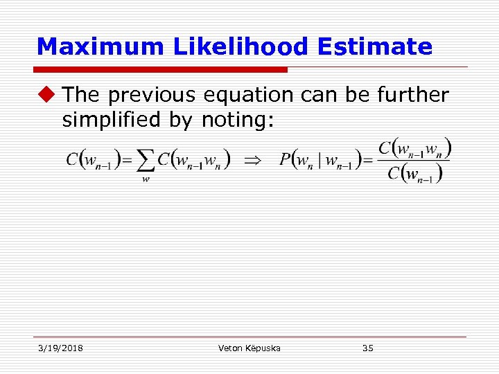 Maximum Likelihood Estimate u The previous equation can be further simplified by noting: 3/19/2018 Veton Këpuska 35
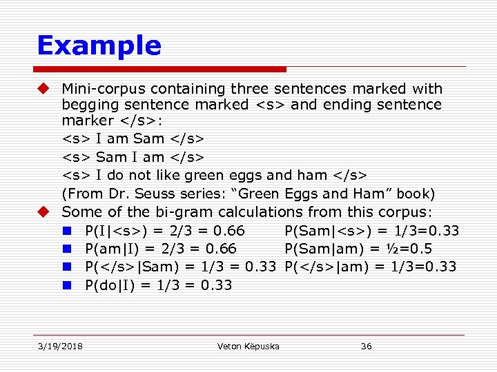 Example u Mini-corpus containing three sentences marked with begging sentence marked
 and ending sentence marker : I am Sam Sam I am I do not like green eggs and ham (From Dr. Seuss series: “Green Eggs and Ham” book) u Some of the bi-gram calculations from this corpus: n P(I|) = 2/3 = 0. 66 P(Sam||am) = 1/3=0. 33 n P(do|I) = 1/3 = 0. 33 3/19/2018 Veton Këpuska 36 ) = 1/3=0. 33 n P(am|I) = 2/3 = 0. 66 P(Sam|am) = ½=0. 5 n P(|Sam) = 1/3 = 0. 33 P(
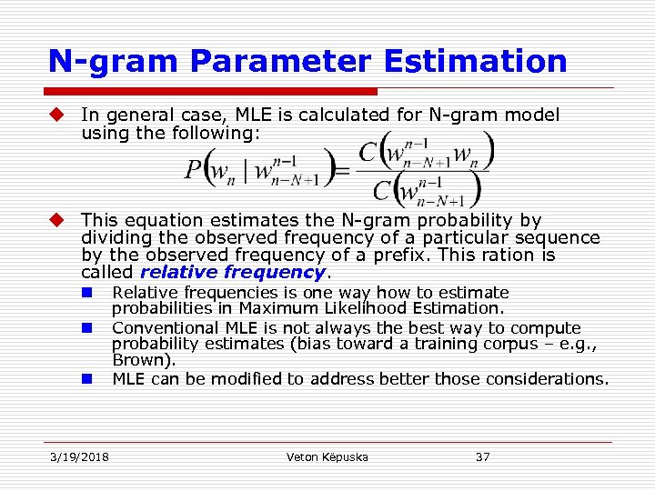 N-gram Parameter Estimation u In general case, MLE is calculated for N-gram model using the following: u This equation estimates the N-gram probability by dividing the observed frequency of a particular sequence by the observed frequency of a prefix. This ration is called relative frequency. n n n 3/19/2018 Relative frequencies is one way how to estimate probabilities in Maximum Likelihood Estimation. Conventional MLE is not always the best way to compute probability estimates (bias toward a training corpus – e. g. , Brown). MLE can be modified to address better those considerations. Veton Këpuska 37
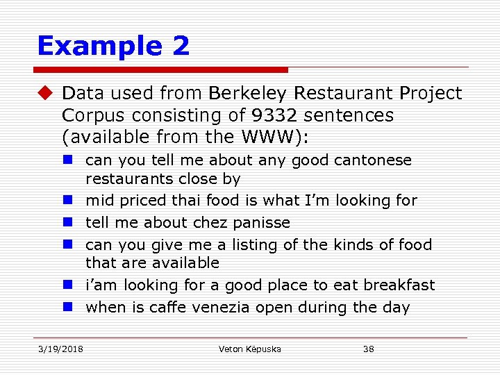 Example 2 u Data used from Berkeley Restaurant Project Corpus consisting of 9332 sentences (available from the WWW): n can you tell me about any good cantonese restaurants close by n mid priced thai food is what I’m looking for n tell me about chez panisse n can you give me a listing of the kinds of food that are available n i’am looking for a good place to eat breakfast n when is caffe venezia open during the day 3/19/2018 Veton Këpuska 38
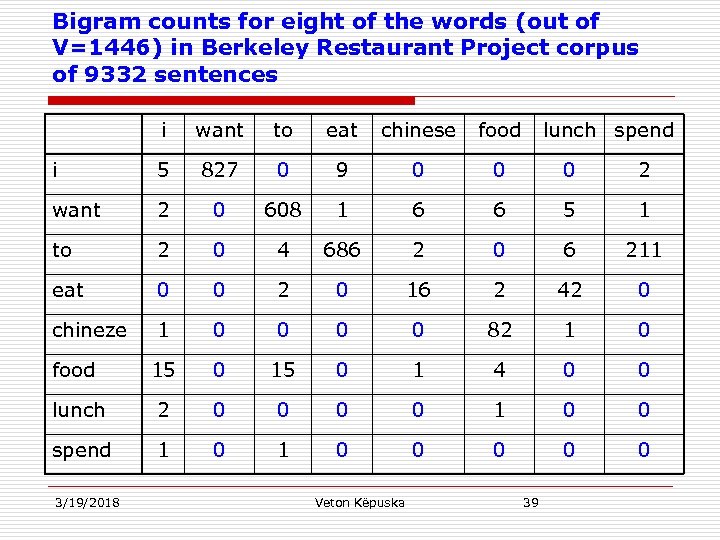 Bigram counts for eight of the words (out of V=1446) in Berkeley Restaurant Project corpus of 9332 sentences i want to eat chinese food i 5 827 0 9 0 0 0 2 want 2 0 608 1 6 6 5 1 to 2 0 4 686 2 0 6 211 eat 0 0 2 0 16 2 42 0 chineze 1 0 0 82 1 0 food 15 0 1 4 0 0 lunch 2 0 0 1 0 0 spend 1 0 0 0 3/19/2018 Veton Këpuska lunch spend 39
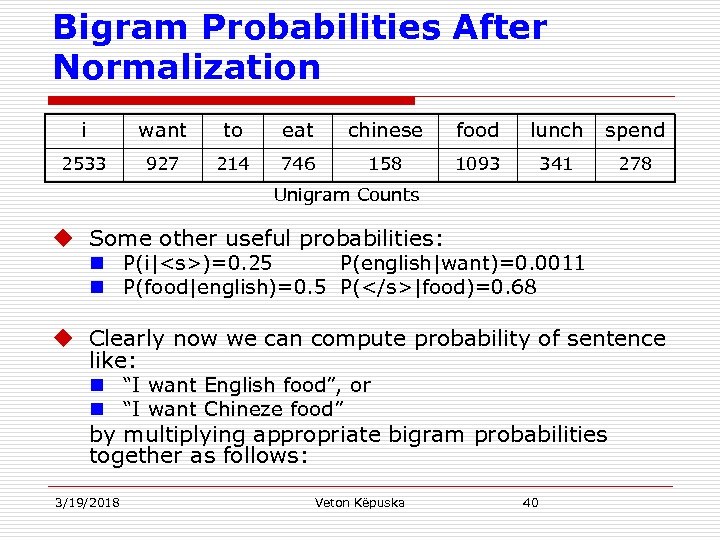 Bigram Probabilities After Normalization i want to eat chinese food lunch spend 2533 927 214 746 158 1093 341 278 Unigram Counts u Some other useful probabilities: n P(i|
)=0. 25 P(english|want)=0. 0011 n P(food|english)=0. 5 P(|food)=0. 68 u Clearly now we can compute probability of sentence like: n “I want English food”, or n “I want Chineze food” by multiplying appropriate bigram probabilities together as follows: 3/19/2018 Veton Këpuska 40
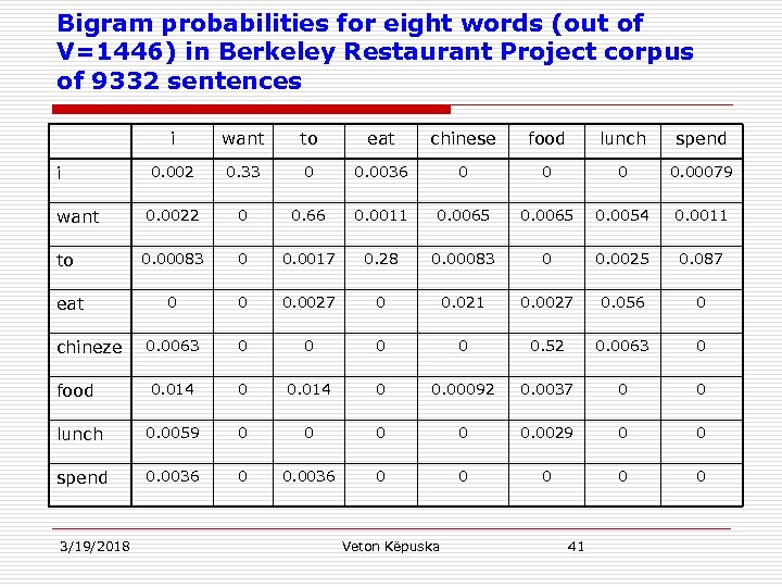 Bigram probabilities for eight words (out of V=1446) in Berkeley Restaurant Project corpus of 9332 sentences i want to eat chinese food lunch spend 0. 002 0. 33 0 0. 0036 0 0. 00079 0. 0022 0 0. 66 0. 0011 0. 0065 0. 0054 0. 0011 0. 00083 0 0. 0017 0. 28 0. 00083 0 0. 0025 0. 087 0 0 0. 0027 0 0. 021 0. 0027 0. 056 0 0. 0063 0 0 0. 52 0. 0063 0 food 0. 014 0 0. 00092 0. 0037 0 0 lunch 0. 0059 0 0 0. 0029 0 0 spend 0. 0036 0 0 0 i want to eat chineze 3/19/2018 Veton Këpuska 41
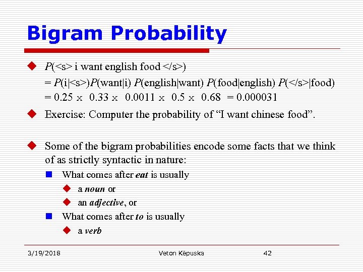 Bigram Probability u P(
 i want english food ) = P(i|)P(want|i) P(english|want) P(food|english) P(|food) = 0. 25 x 0. 33 x 0. 0011 x 0. 5 x 0. 68 = 0. 000031 u Exercise: Computer the probability of “I want chinese food”. u Some of the bigram probabilities encode some facts that we think of as strictly syntactic in nature: n What comes after eat is usually u a noun or u an adjective, or n What comes after to is usually u a verb 3/19/2018 Veton Këpuska 42
 Trigram Modeling u Although we will generally show bigram models in this chapter for pedagogical purposes, note that when there is sufficient training data we are more likely to use trigram models, which condition on the previous two words rather than the previous word. n To compute trigram probabilities at the very beginning of sentence, we can use two pseudo-words for the first trigram (i. e. , P(I|
). 3/19/2018 Veton Këpuska 43
 Training and Test Sets u N-gram models are obtained from a corpus that is trained on. u Those models are used on some new data in some task (e. g. speech recognition). n New data or task will not be exactly the same as data that was used for training. u Formally: n Data that is used to build the N-gram (or any model) are called Training Set or Training Corpus n Data that are used to test the models comprise Test Set or Test Corpus. 3/19/2018 Veton Këpuska 44
 Model Evaluation u Training-and-testing paradigm can also be used to evaluate different N-gram architectures: n n Comparing N-grams of different order N, or Using the different smoothing algorithms (to be introduced later) u Train various models using training corpus u Evaluate each model on the test corpus. u How do we measure the performance of each model on the test corpus? n Perplexity (introduced latter in the chapter) – computing probability of each sentence in the test set: the model that assigns a higher probability to the test set (hence more accurately predicts the test set) is assumed to be a better model. u Because evaluation metric is based on test set probability, it’s important not to let the test sentences into the training set. Avoiding training on the test set data. 3/19/2018 Veton Këpuska 45
 Other Divisions of Data u Extra source of data to augment the training set is needed. This data is called a held-out set. n N-gram model is based on only training set. n Held-out set is used to set additional (other) parameters of our model. u Used to set interpolation parameters of N-gram model u Multiple test sets: n Test set that is used often in measuring performance of the model typically is called development (test) set. n Due to its high usage the models may be tuned to it. Thus a new completely unseen (or seldom used data set) should be used for final evaluation. This set is called evaluation (test) set. 3/19/2018 Veton Këpuska 46
 Picking Train, Development Test and Evaluation Test Data u For training we need as much data as possible. u However, for Testing we need sufficient data in order for the resulting measurements to be statistically significant. u In practice often the data is divided into 80% training 10% development and 10% evaluation. 3/19/2018 Veton Këpuska 47
 N-gram Sensitivity to the Training Corpus. 1. N-gram modeling, like many statistical models, is very dependent on the training corpus. u Often the model encodes very specific facts about a given training corpus. 2. N-grams do a better and better job of modeling the training corpus as we increase the value of N. u This is another aspect of model being tuned to specifically to training data at the expense of generality. 3/19/2018 Veton Këpuska 48
 Visualization of N-gram Modeling u Shannon (1951) AND Miller & Selfridge (1950). u The simplest way to visualize how this works is for the unigram case: n n All words of English language covering the probability space between 0 and 1 – each word thus covering an interval of size equal to its (relative) frequency. Let us choose a random number between 0 and 1, and print out the word whose interval includes the real value we have chosen. We continue choosing random numbers and generating words until we randomly generate the sentence-final token . The same technique can be used to generate bigrams by u first generating a random bigram that starts with
 (according to its bigram probability) u Then choosing a random bigram to follow it (again according to its conditional probability), and so on. 3/19/2018 Veton Këpuska 49
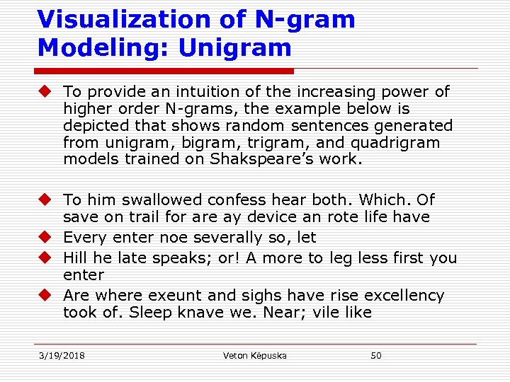 Visualization of N-gram Modeling: Unigram u To provide an intuition of the increasing power of higher order N-grams, the example below is depicted that shows random sentences generated from unigram, bigram, trigram, and quadrigram models trained on Shakspeare’s work. u To him swallowed confess hear both. Which. Of save on trail for are ay device an rote life have u Every enter noe severally so, let u Hill he late speaks; or! A more to leg less first you enter u Are where exeunt and sighs have rise excellency took of. Sleep knave we. Near; vile like 3/19/2018 Veton Këpuska 50
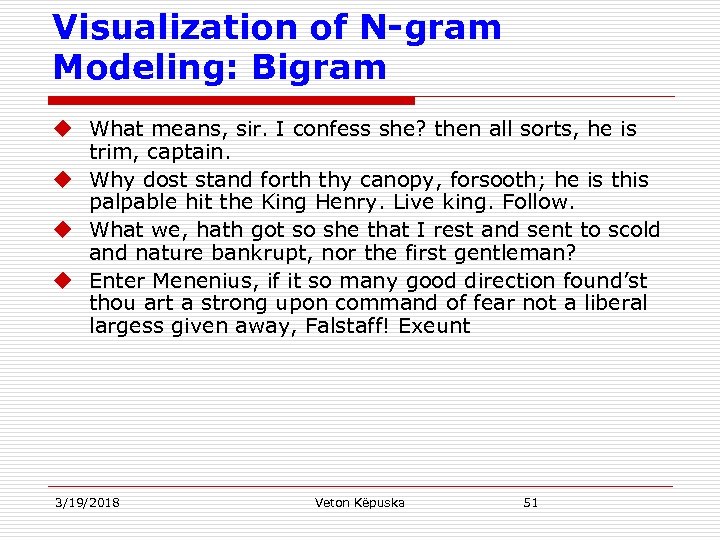 Visualization of N-gram Modeling: Bigram u What means, sir. I confess she? then all sorts, he is trim, captain. u Why dost stand forth thy canopy, forsooth; he is this palpable hit the King Henry. Live king. Follow. u What we, hath got so she that I rest and sent to scold and nature bankrupt, nor the first gentleman? u Enter Menenius, if it so many good direction found’st thou art a strong upon command of fear not a liberal largess given away, Falstaff! Exeunt 3/19/2018 Veton Këpuska 51
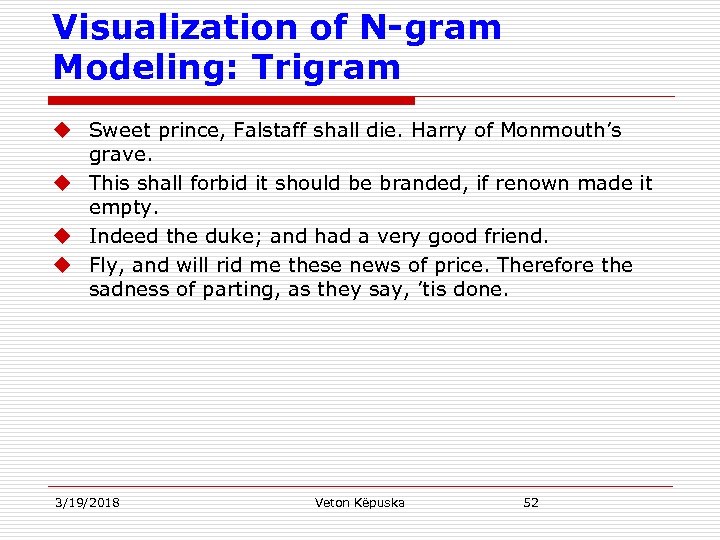 Visualization of N-gram Modeling: Trigram u Sweet prince, Falstaff shall die. Harry of Monmouth’s grave. u This shall forbid it should be branded, if renown made it empty. u Indeed the duke; and had a very good friend. u Fly, and will rid me these news of price. Therefore the sadness of parting, as they say, ’tis done. 3/19/2018 Veton Këpuska 52
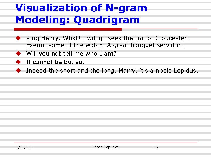 Visualization of N-gram Modeling: Quadrigram u King Henry. What! I will go seek the traitor Gloucester. Exeunt some of the watch. A great banquet serv’d in; u Will you not tell me who I am? u It cannot be but so. u Indeed the short and the long. Marry, ’tis a noble Lepidus. 3/19/2018 Veton Këpuska 53
 Size of N in N-gram Models u The longer the context on which we train the model, the more coherent the sentences. n In the unigram sentences, there is no coherent relation between words, nor sentence-final punctuation. n The bigram sentences have some very local word-toword coherence (especially if we consider that punctuation counts as a word). n The trigram and quadrigram sentences are beginning to look a lot like Shakespeare. n Indeed a careful investigation of the quadrigram sentences shows that they look a little too much like Shakespeare. The words It cannot be but so are directly from King John. 3/19/2018 Veton Këpuska 54
 Specificity vs Generality u The variability of words phrases in Shakespeare is not very large in the context of training corpora used for language modeling: n N = 884, 647 & V = 29, 066 n N-gram probability matrices are very sparse: u V 2 = 844, 000 possible bigrams alone u V 4 = 7 x 10¹⁷ number of possible quadrigrams. n Once the generator has chosen the first quadrigram, there are only five possible continuations (that, I , he, thou, and so). In fact for many quadrigrams there is only one continuation. 3/19/2018 Veton Këpuska 55
 Dependence of Grammar to its Training Set. u Example of Wall Street Journal (WSJ) Corpus based on the newspaper. u Shakespeare work and WSJ are both in English, so one might expect some overlap between our N-grams for the two genres. n In order to check whether this is true the next slides provide sentences generated by unigram, bigram and trigrammars trained on 40 million words from WSJ. 3/19/2018 Veton Këpuska 56
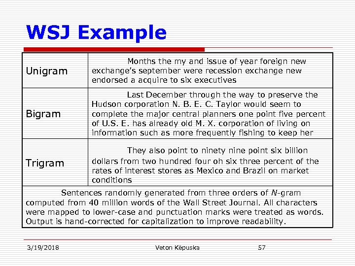 WSJ Example Unigram Months the my and issue of year foreign new exchange’s september were recession exchange new endorsed a acquire to six executives Bigram Last December through the way to preserve the Hudson corporation N. B. E. C. Taylor would seem to complete the major central planners one point five percent of U. S. E. has already old M. X. corporation of living on information such as more frequently fishing to keep her Trigram They also point to ninety nine point six billion dollars from two hundred four oh six three percent of the rates of interest stores as Mexico and Brazil on market conditions Sentences randomly generated from three orders of N-gram computed from 40 million words of the Wall Street Journal. All characters were mapped to lower-case and punctuation marks were treated as words. Output is hand-corrected for capitalization to improve readability. 3/19/2018 Veton Këpuska 57
 Comparison of Shakespeare and WSJ Examples u While superficially they both seem to model “English-like sentences” there is obviously no overlap whatsoever in possible sentences, and little if any overlap even in small phrases. This stark difference tells us that statistical models are likely to be pretty useless as predictors if the training sets and the test sets are as different as Shakespeare and WSJ. u How should we deal with this problem when we build Ngram models? 3/19/2018 Veton Këpuska 58
 Comparison of Shakespeare and WSJ Examples n n n 3/19/2018 In general we need to be sure to use a training corpus that looks like our test corpus. We especially wouldn’t choose training and tests from different genres of text like newspaper text, early English fiction, telephone conversations, and web pages. Sometimes finding appropriate training text for a specific new task can be difficult; to build N-grams for text prediction in SMS (Short Message Service), we need a training corpus of SMS data. To build N-grams on business meetings, we would need to have corpora of transcribed business meetings. For general research where we know we want written English but don’t have a domain in mind, we can use a balanced training corpus that includes cross-sections from different genres, such as the 1 -million word Brown corpus of English (Francis and Kuˇcera, 1982) or the 100 -million word British National Corpus (Leech et al. , 1994). Recent research has also studied ways to dynamically adapt language models to different genres; Veton Këpuska 59
 Unknown Words: Open vs. Closed Vocabulary Tasks u Sometimes we have a language task in which we know all the words that can occur, and hence we know the vocabulary size V in advance. n The closed vocabulary assumption is the assumption that we have such a lexicon, and that the test set can only contain words from this lexicon. The closed vocabulary task thus assumes there are no unknown words. 3/19/2018 Veton Këpuska 60
 Unknown Words: Open vs. Closed Vocabulary Tasks u As we suggested earlier, the number of unseen words grows constantly, so we can’t possibly know in advance exactly how many there are, and we’d like our model to do something reasonable with them. We call these OOV unseen events unknown words, or out of vocabulary (OOV) words. The percentage of OOV words that appear in the test set is called the OOV rate. n An open vocabulary system is one where we model these potential unknown words in the test set by adding a pseudo-word called
 Training Probabilities of Unknown Model u We can train the probabilities of the unknown word model
 Evaluating N-Grams Perplexity
 Perplexity u The correct way to evaluate the performance of a language model is to embed it in an application and measure the total performance of the application. n Such end-to end evaluation, also called in vivo evaluation, is the only way to know if a particular improvement in a component is really going to help the task at hand. n Thus for speech recognition, we can compare the performance of two language models by running the speech recognizer twice, once with each language model, and seeing which gives the more accurate transcription. 3/19/2018 Veton Këpuska 64
 Perplexity u End-to-end evaluation is often very expensive; evaluating a large speech recognition test set, for example, takes hours or even days. n Thus we would like a metric that can be used to quickly evaluate potential improvements in a language model. n Perplexity is the most common evaluation metric for N-gram language models. While an improvement in perplexity does not guarantee an improvement in speech recognition performance (or any other end-toend metric), it often correlates with such improvements. n Thus it is commonly used as a quick check on an algorithm; an improvement in perplexity can then be confirmed by an end-to-end evaluation. 3/19/2018 Veton Këpuska 65
 Perplexity u Given two probabilistic models, n the better model is the one that has a tighter fit to the test data, or n predicts the details of the test data better. u We can measure better prediction by looking at the probability the model assigns to the test data; n the better model will assign a higher probability to the test data. 3/19/2018 Veton Këpuska 66
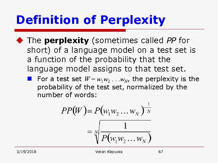 Definition of Perplexity u The perplexity (sometimes called PP for short) of a language model on a test set is a function of the probability that the language model assigns to that test set. n For a test set W = w 1 w 2. . . w. N, the perplexity is the probability of the test set, normalized by the number of words: 3/19/2018 Veton Këpuska 67
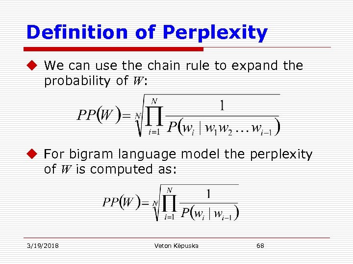 Definition of Perplexity u We can use the chain rule to expand the probability of W: u For bigram language model the perplexity of W is computed as: 3/19/2018 Veton Këpuska 68
 Interpretation of Perplexity 1. Minimizing perplexity is equivalent to maximizing the test set probability according to the language model. u What we generally use for word sequence in the general Equation presented in previous slide is the entire sequence of words in some test set. n Since this sequence will cross many sentence boundaries, we need to include u the begin-and end-sentence markers
 and in the probability computation. u also need to include the end-of-sentence marker (but not the beginning-of-sentence marker ) in the total count of word tokens N. 3/19/2018 Veton Këpuska 69
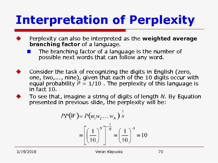 Interpretation of Perplexity u u u Perplexity can also be interpreted as the weighted average branching factor of a language. n The branching factor of a language is the number of possible next words that can follow any word. Consider the task of recognizing the digits in English (zero, one, two, . . . , nine), given that each of the 10 digits occur with equal probability P = 1/10. The perplexity of this language is in fact 10. To see that, imagine a string of digits of length N. By Equation presented in previous slide, the perplexity will be: 3/19/2018 Veton Këpuska 70
 Interpretation of Perplexity u Exercise: Suppose that the number zero is really frequent and occurs 10 times more often than other numbers. n Show that the perplexity to be lower, as expected since most of the time the next number will be zero. n Branching factor however, is still the same for digit recognition task (e. g. 10). 3/19/2018 Veton Këpuska 71
 Interpretation of Perplexity u Perplexity is also related to the information theoretic notion of entropy as it will be shown latter in this chapter. 3/19/2018 Veton Këpuska 72
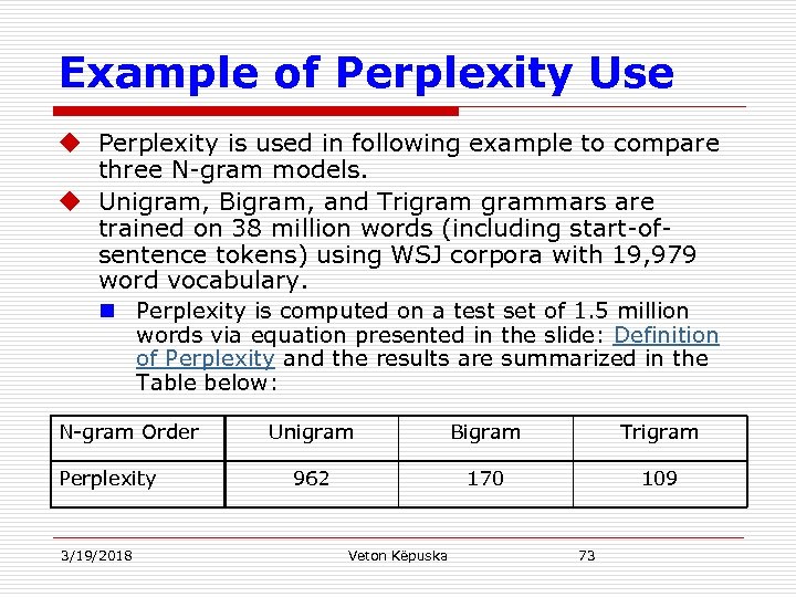 Example of Perplexity Use u Perplexity is used in following example to compare three N-gram models. u Unigram, Bigram, and Trigrammars are trained on 38 million words (including start-ofsentence tokens) using WSJ corpora with 19, 979 word vocabulary. n Perplexity is computed on a test set of 1. 5 million words via equation presented in the slide: Definition of Perplexity and the results are summarized in the Table below: N-gram Order Perplexity 3/19/2018 Unigram Bigram Trigram 962 170 109 Veton Këpuska 73
 Example of Perplexity Use u As we see in previous slide, the more information the Ngram gives us about the word sequence, the lower the perplexity: n the perplexity is related inversely to the likelihood of the test sequence according to the model. u Note that in computing perplexities the N-gram model P must be constructed without any knowledge of the test set t. Any kind of knowledge of the test set can cause the perplexity to be artificially low. u For example, we defined above the closed vocabulary task, in which the vocabulary for the test set is specified in advance. This can greatly reduce the perplexity. As long as this knowledge is provided equally to each of the models we are comparing, the closed vocabulary perplexity can still be useful for comparing models, but care must be taken in interpreting the results. In general, the perplexity of two language models is only comparable if they use the same vocabulary. 3/19/2018 Veton Këpuska 74
 Smoothing
 Smoothing u There is a major problem with the maximum likelihood estimation process we have seen for training the parameters of an N-gram model. This is the problem of sparse data caused by the fact that our maximum likelihood estimate was based on a particular set of training data. For any N-gram that occurred a sufficient number of times, we might have a good estimate of its probability. But because any corpus is limited, some perfectly acceptable English word sequences are bound to be missing from it. 1. This missing data means that the N-gram matrix for any given training corpus is bound to have a very large number of cases of putative “zero probability N-grams” that should really have some non-zero probability. 2. Furthermore, the MLE method also produces poor estimates when the counts are non-zero but still small. n 3/19/2018 Veton Këpuska 76
 Smoothing u We need a method which can help get better estimates for these zero or low frequency counts. n Zero counts turn out to cause another huge problem. u The perplexity metric defined above requires that we compute the probability of each test sentence. u But if a test sentence has an N-gram that never appeared in the training set, the Maximum Likelihood estimate of the probability for this N-gram, and hence for the whole test sentence, will be zero! u This means that in order to evaluate our language models, we need to modify the MLE method to assign some non-zero probability to any N-gram, even one that was never observed in training. 3/19/2018 Veton Këpuska 77
 Smoothing u The term smoothing is used for such modifications that address the poor estimates due to variability in small data sets. n The name comes from the fact that (looking ahead a bit) we will be shaving a little bit of probability mass from the higher counts, and piling it instead on the zero counts, making the distribution a little less discontinuous. u In the next few sections some smoothing algorithms are introduced. u The original Berkeley Restaurant example introduced previously will be used to show smoothing algorithms modify the bigram probabilities. 3/19/2018 Veton Këpuska 78
 Laplace Smoothing u One simple way to do smoothing is to take our matrix of bigram counts, before we normalize them into probabilities, and add one to all the counts. This algorithm is called Laplace smoothing, or Laplace’s Law. u Laplace smoothing does not perform well enough to be used in modern N-gram models, but we begin with it because it introduces many of the concepts that we will see in other smoothing algorithms, and also gives us a useful baseline. 3/19/2018 Veton Këpuska 79
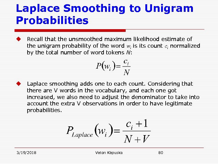 Laplace Smoothing to Unigram Probabilities u Recall that the unsmoothed maximum likelihood estimate of the unigram probability of the word wi is its count ci normalized by the total number of word tokens N: u Laplace smoothing adds one to each count. Considering that there are V words in the vocabulary, and each one got increased, we also need to adjust the denominator to take into account the extra V observations in order to have legitimate probabilities. 3/19/2018 Veton Këpuska 80
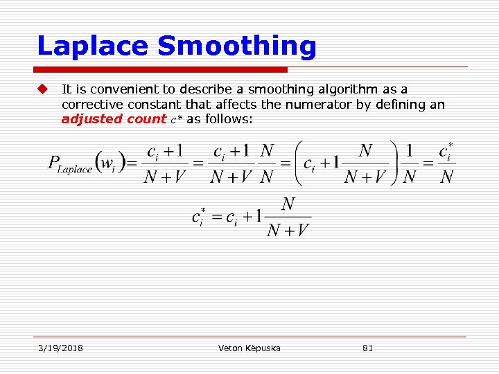 Laplace Smoothing u It is convenient to describe a smoothing algorithm as a corrective constant that affects the numerator by defining an adjusted count c* as follows: 3/19/2018 Veton Këpuska 81
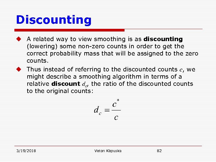 Discounting u A related way to view smoothing is as discounting (lowering) some non-zero counts in order to get the correct probability mass that will be assigned to the zero counts. u Thus instead of referring to the discounted counts c, we might describe a smoothing algorithm in terms of a relative discount dc, the ratio of the discounted counts to the original counts: 3/19/2018 Veton Këpuska 82
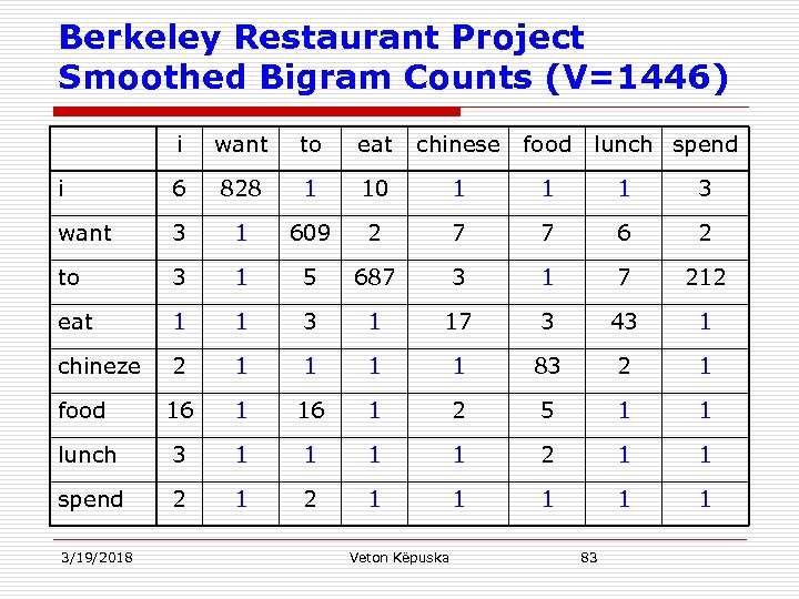 Berkeley Restaurant Project Smoothed Bigram Counts (V=1446) i want to eat chinese food i 6 828 1 10 1 1 1 3 want 3 1 609 2 7 7 6 2 to 3 1 5 687 3 1 7 212 eat 1 1 3 1 17 3 43 1 chineze 2 1 1 83 2 1 food 16 1 2 5 1 1 lunch 3 1 1 2 1 1 spend 2 1 1 1 3/19/2018 Veton Këpuska lunch spend 83
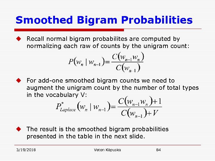 Smoothed Bigram Probabilities u Recall normal bigram probabilites are computed by normalizing each raw of counts by the unigram count: u For add-one smoothed bigram counts we need to augment the unigram count by the number of total types in the vocabulary V: u The result is the smoothed bigram probabilities presented in the table in the next slide. 3/19/2018 Veton Këpuska 84
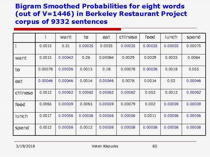 Bigram Smoothed Probabilities for eight words (out of V=1446) in Berkeley Restaurant Project corpus of 9332 sentences i want to eat chinese food lunch spend i 0. 0015 0. 21 0. 00025 0. 00075 want 0. 0013 0. 00042 0. 26 0. 00084 0. 0029 0. 0025 0. 0084 to 0. 00078 0. 00026 0. 0013 0. 18 0. 00078 0. 00026 0. 0018 0. 055 eat 0. 00046 0. 0014 0. 00046 0. 0078 0. 0014 0. 02 0. 00046 chinese 0. 0012 0. 00062 0. 052 0. 0012 0. 00062 food 0. 0063 0. 00039 0. 00079 0. 002 0. 00039 lunch 0. 0017 0. 00056 0. 0011 0. 00056 spend 0. 0012 0. 00058 3/19/2018 Veton Këpuska 85
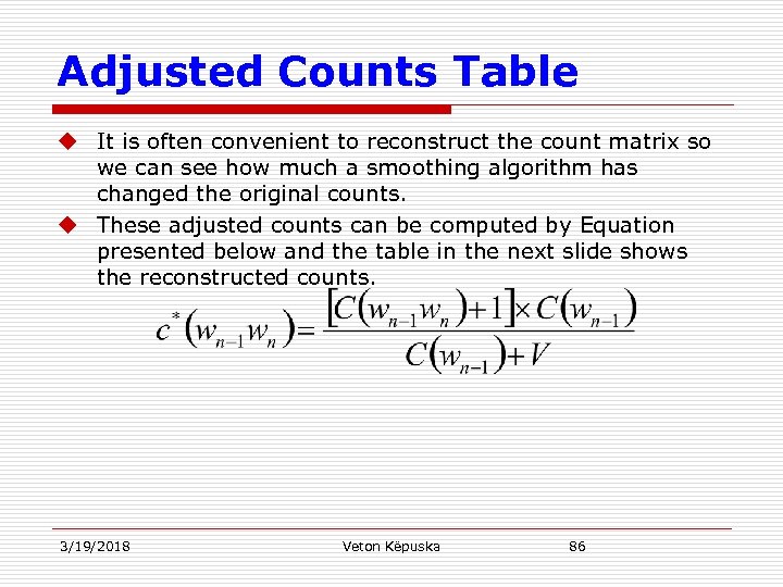 Adjusted Counts Table u It is often convenient to reconstruct the count matrix so we can see how much a smoothing algorithm has changed the original counts. u These adjusted counts can be computed by Equation presented below and the table in the next slide shows the reconstructed counts. 3/19/2018 Veton Këpuska 86
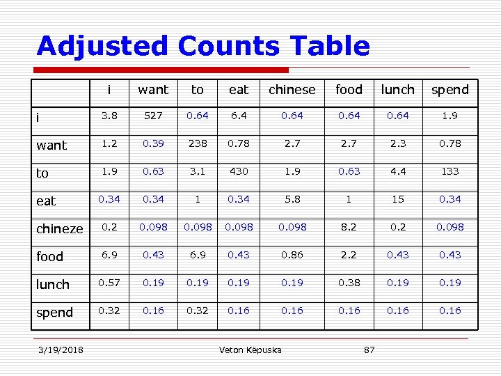 Adjusted Counts Table i want to eat chinese food lunch spend i 3. 8 527 0. 64 6. 4 0. 64 1. 9 want 1. 2 0. 39 238 0. 78 2. 7 2. 3 0. 78 to 1. 9 0. 63 3. 1 430 1. 9 0. 63 4. 4 133 0. 34 1 0. 34 5. 8 1 15 0. 34 chineze 0. 2 0. 098 8. 2 0. 098 food 6. 9 0. 43 0. 86 2. 2 0. 43 lunch 0. 57 0. 19 0. 38 0. 19 spend 0. 32 0. 16 eat 3/19/2018 Veton Këpuska 87
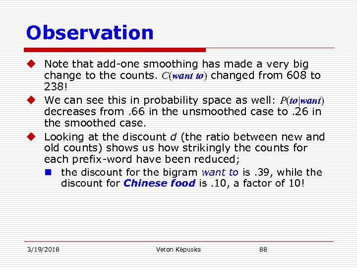 Observation u Note that add-one smoothing has made a very big change to the counts. C(want to) changed from 608 to 238! u We can see this in probability space as well: P(to|want) decreases from. 66 in the unsmoothed case to. 26 in the smoothed case. u Looking at the discount d (the ratio between new and old counts) shows us how strikingly the counts for each prefix-word have been reduced; n the discount for the bigram want to is. 39, while the discount for Chinese food is. 10, a factor of 10! 3/19/2018 Veton Këpuska 88
 Problems with Add-One (Laplace) Smoothing u The sharp change in counts and probabilities occurs because too much probability mass is moved to all the zeros. n We could move a bit less mass by adding a fractional count rather than 1 (add-d smoothing; (Lidstone, 1920; Jeffreys, 1948)), but n this method requires a method for choosing d dynamically, results in an inappropriate discount for many counts, and turns out to give counts with poor variances. n For these and other reasons (Gale and Church, 1994), we’ll need use better smoothing methods for N-grams like the ones we will present in the next section. 3/19/2018 Veton Këpuska 89
 Good-Turing Discounting u A number of much better algorithms have been developed that are only slightly more complex than add-one smoothing: Good-Turing u The idea behind a number of those algorithms is to use the count of things you’ve seen once to help estimate the count of things you have never seen. u Good described the algorithm in 1953 in which he credits Turing for the original idea. u Basic idea in this algorithm is to re-estimate the amount of probability mass t assign to N-grams with zero counts by looking at the number of N-grams that occurred only one time. n n 3/19/2018 A word or N-gram that occurs once is called a singleton. Good-Turing algorithm uses the frequency of singletons as a re -estimate of the frequency of zero-count bigrams. Veton Këpuska 90
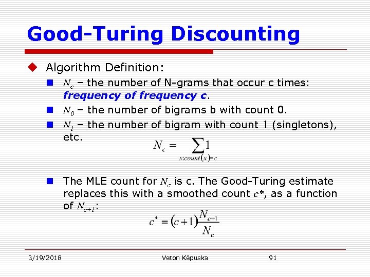 Good-Turing Discounting u Algorithm Definition: n Nc – the number of N-grams that occur c times: frequency of frequency c. n N 0 – the number of bigrams b with count 0. n N 1 – the number of bigram with count 1 (singletons), etc. n The MLE count for Nc is c. The Good-Turing estimate replaces this with a smoothed count c*, as a function of Nc+1: 3/19/2018 Veton Këpuska 91
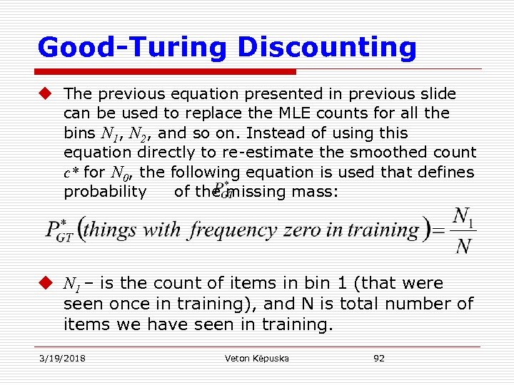 Good-Turing Discounting u The previous equation presented in previous slide can be used to replace the MLE counts for all the bins N 1, N 2, and so on. Instead of using this equation directly to re-estimate the smoothed count c* for N 0, the following equation is used that defines probability of the missing mass: u N 1 – is the count of items in bin 1 (that were seen once in training), and N is total number of items we have seen in training. 3/19/2018 Veton Këpuska 92
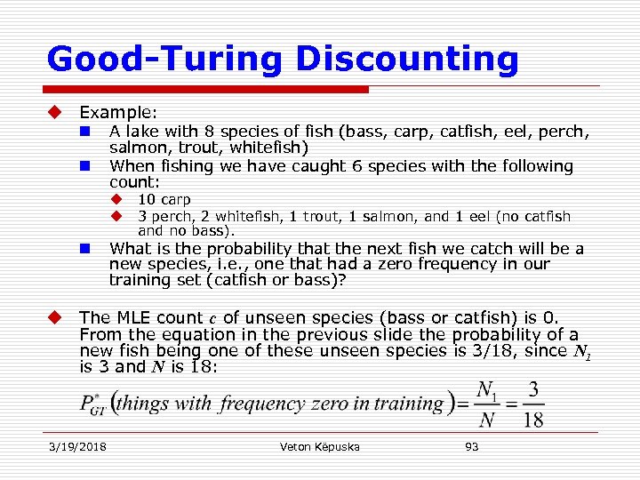 Good-Turing Discounting u Example: n n A lake with 8 species of fish (bass, carp, catfish, eel, perch, salmon, trout, whitefish) When fishing we have caught 6 species with the following count: u 10 carp u 3 perch, 2 whitefish, 1 trout, 1 salmon, and 1 eel (no catfish and no bass). n What is the probability that the next fish we catch will be a new species, i. e. , one that had a zero frequency in our training set (catfish or bass)? u The MLE count c of unseen species (bass or catfish) is 0. From the equation in the previous slide the probability of a new fish being one of these unseen species is 3/18, since N 1 is 3 and N is 18: 3/19/2018 Veton Këpuska 93
 Good-Turing Discounting: Example u Lets now estimate the probability that the next fish will be another trout? MLE count for trout is 1, so the MLE estimated probability is 1/18. u However, the Good-Turing estimate must be lower, since we took 3/18 of our probability mass to use on unseen events! n Must discount MLE probabilities for observed counts (perch, whitefish, trout, salmon, and eel) u The revised count c* and Good-Turing smoothed probabilities for species with counts 0 (like bass or catfish in previous example) or counts 1 (like trout, salmon, or eel) are as follows: 3/19/2018 Veton Këpuska 94
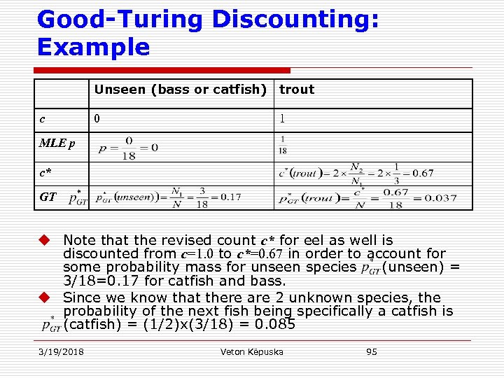 Good-Turing Discounting: Example Unseen (bass or catfish) trout c 0 1 MLE p c* GT u Note that the revised count c* for eel as well is discounted from c=1. 0 to c*=0. 67 in order to account for some probability mass for unseen species (unseen) = 3/18=0. 17 for catfish and bass. u Since we know that there are 2 unknown species, the probability of the next fish being specifically a catfish is (catfish) = (1/2)x(3/18) = 0. 085 3/19/2018 Veton Këpuska 95
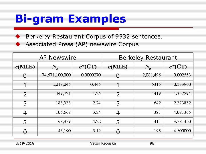 Bi-gram Examples u Berkeley Restaurant Corpus of 9332 sentences. u Associated Press (AP) newswire Corpus AP Newswire c(MLE) Nc Berkeley Restaurant c*(GT) c(MLE) Nc c*(GT) 0 74, 671, 100, 000 0. 0000270 0 2, 081, 496 0. 002553 1 2, 018, 046 0. 446 1 5315 0. 533960 2 449, 721 1. 26 2 1419 1. 357294 3 188, 933 2. 24 3 642 2. 373832 4 105, 668 3. 24 4 381 4. 081365 5 68, 379 4. 22 5 311 3. 781350 6 48, 190 5. 19 6 196 4. 500000 3/19/2018 Veton Këpuska 96
 Advanced Issues in Good. Turing Estimation u Assumptions of Good-Turing Estimation: n Distribution of each bigram is binomial n The number N 0 of bigrams that have not been seen is known. u This number is known if size V of vocabulary is known ⇒ total number of bigrams is thus V 2. u The raw number Nc can not be used since re-estimate c* for Nc dependents on Nc+1 and the re-estimation expression is undefined when Nc+1=0. n In the example of the fish species N 4 = 0, thus how can one compute N 3? ⇒ Simple Good-Turing Algorithm 3/19/2018 Veton Këpuska 97
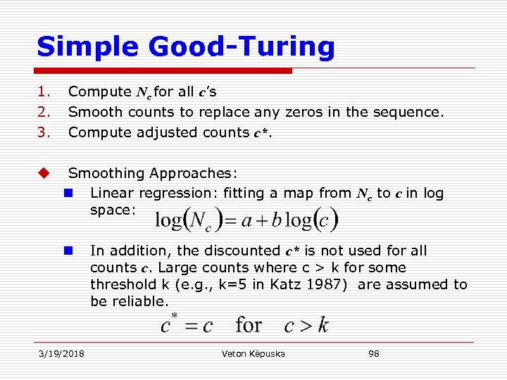 Simple Good-Turing 1. 2. 3. Compute Nc for all c’s Smooth counts to replace any zeros in the sequence. Compute adjusted counts c*. u Smoothing Approaches: n Linear regression: fitting a map from Nc to c in log space: n 3/19/2018 In addition, the discounted c* is not used for all counts c. Large counts where c > k for some threshold k (e. g. , k=5 in Katz 1987) are assumed to be reliable. Veton Këpuska 98
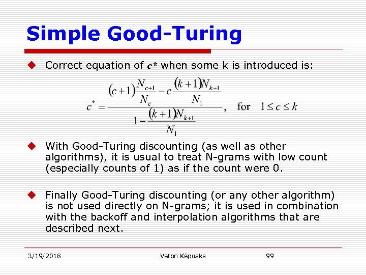 Simple Good-Turing u Correct equation of c* when some k is introduced is: u With Good-Turing discounting (as well as other algorithms), it is usual to treat N-grams with low count (especially counts of 1) as if the count were 0. u Finally Good-Turing discounting (or any other algorithm) is not used directly on N-grams; it is used in combination with the backoff and interpolation algorithms that are described next. 3/19/2018 Veton Këpuska 99
 Interpolation
 Interpolation u Discounting algorithms can help solve the problem of zero frequency N-grams. u Additional knowledge that is not used: n If trying to compute P(wn|wn-1 wn-2) but we have no examples of a particular trigram wn-2 wn-1 wn n Estimate trigram probability based on the bigram probability P(wn|wn-1). n If there are no counts for computation of bigram probability P(wn|wn-1), use unigram probability P(wn). u There are two ways to rely on this N-gram “hiearchy”: n Backoff, and n Interpolation 3/19/2018 Veton Këpuska 101
 Backoff vs. Interpolation u Backoff: n Relies solely on the trigram counts. When there is a zero count evidence of a trigram then the backoff to lower Ngram. u Interpolation: n Probability estimates are always mixed from all N-gram estimators: u Weighted interpolation of trigram, bigram and unigram counts. u Simple Interpolation – Linear Interpolation 3/19/2018 Veton Këpuska 102
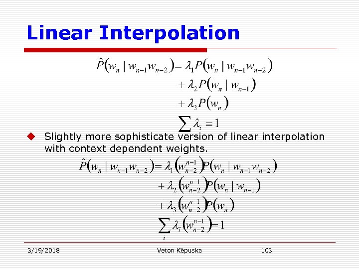 Linear Interpolation u Slightly more sophisticate version of linear interpolation with context dependent weights. 3/19/2018 Veton Këpuska 103
 Computing Interpolation Weights l u Weights are set from held-out corpus. n Held-out corpus is additional training corpus that is NOT used to set the N-gram counts but to set other parameters like in this case. u Choosing l values that maximize the estimated interpolated probability for example with EM algorithm (iterative algorithm discussed in latter chapters). 3/19/2018 Veton Këpuska 104
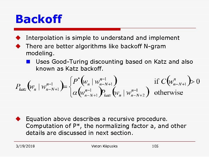 Backoff u Interpolation is simple to understand implement u There are better algorithms like backoff N-gram modeling. n Uses Good-Turing discounting based on Katz and also known as Katz backoff. u Equation above describes a recursive procedure. Computation of P*, the normalizing factor a, and other details are discussed in next section. 3/19/2018 Veton Këpuska 105
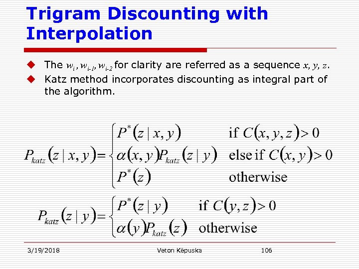 Trigram Discounting with Interpolation u The wi , wi-1, wi-2 for clarity are referred as a sequence x, y, z. u Katz method incorporates discounting as integral part of the algorithm. 3/19/2018 Veton Këpuska 106
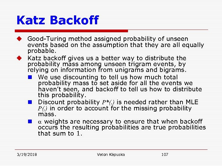 Katz Backoff u Good-Turing method assigned probability of unseen events based on the assumption that they are all equally probable. u Katz backoff gives us a better way to distribute the probability mass among unseen trigram events, by relying on information from unigrams and bigrams. n We use discounting to tell us how much total probability mass to set aside for all the events we haven’t seen, and backoff to tell us how to distribute this probability. n Discount probability P*(. ) is needed rather than MLE P(. ) in order to account for the missing probability mass. n a weights are necessary to ensure that when backoff occurs the resulting probabilities are true probabilities that sum to 1. 3/19/2018 Veton Këpuska 107
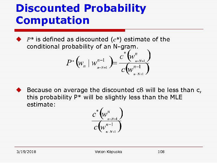 Discounted Probability Computation u P* is defined as discounted (c*) estimate of the conditional probability of an N-gram. u Because on average the discounted c 8 will be less than c, this probability P* will be slightly less than the MLE estimate: 3/19/2018 Veton Këpuska 108
 Discounted Probability Computation u The previous slide computation will leave some probability mass for the lower order N-grams, which is then distributed by the a weights (descirbed in next section). u The table in the next slide shows the result of Katz backoff bigram probabilities for previous 8 sample words computed from Be. RP corpus using the SRILM toolkit. 3/19/2018 Veton Këpuska 109
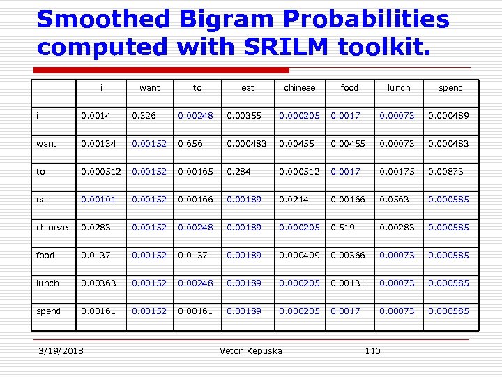 Smoothed Bigram Probabilities computed with SRILM toolkit. i want to eat chinese food lunch spend i 0. 0014 0. 326 0. 00248 0. 00355 0. 000205 0. 0017 0. 00073 0. 000489 want 0. 00134 0. 00152 0. 656 0. 000483 0. 00455 0. 00073 0. 000483 to 0. 000512 0. 00152 0. 00165 0. 284 0. 000512 0. 00175 0. 00873 eat 0. 00101 0. 00152 0. 00166 0. 00189 0. 0214 0. 00166 0. 0563 0. 000585 chineze 0. 0283 0. 00152 0. 00248 0. 00189 0. 000205 0. 519 0. 00283 0. 000585 food 0. 0137 0. 00152 0. 0137 0. 00189 0. 000409 0. 00366 0. 00073 0. 000585 lunch 0. 00363 0. 00152 0. 00248 0. 00189 0. 000205 0. 00131 0. 00073 0. 000585 spend 0. 00161 0. 00152 0. 00161 0. 00189 0. 000205 0. 0017 0. 00073 0. 000585 3/19/2018 Veton Këpuska 110
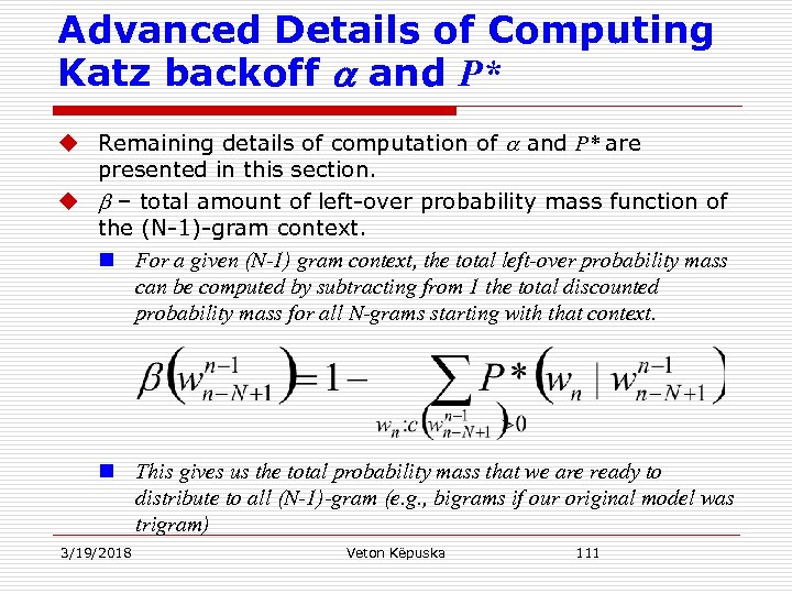 Advanced Details of Computing Katz backoff a and P* u Remaining details of computation of a and P* are presented in this section. u b – total amount of left-over probability mass function of the (N-1)-gram context. n For a given (N-1) gram context, the total left-over probability mass can be computed by subtracting from 1 the total discounted probability mass for all N-grams starting with that context. n This gives us the total probability mass that we are ready to distribute to all (N-1)-gram (e. g. , bigrams if our original model was trigram) 3/19/2018 Veton Këpuska 111
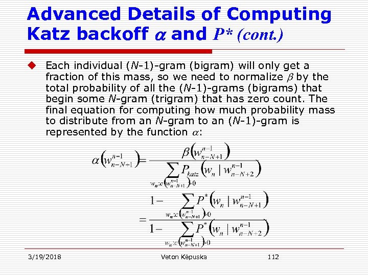 Advanced Details of Computing Katz backoff a and P* (cont. ) u Each individual (N-1)-gram (bigram) will only get a fraction of this mass, so we need to normalize b by the total probability of all the (N-1)-grams (bigrams) that begin some N-gram (trigram) that has zero count. The final equation for computing how much probability mass to distribute from an N-gram to an (N-1)-gram is represented by the function a: 3/19/2018 Veton Këpuska 112
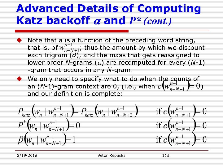 Advanced Details of Computing Katz backoff a and P* (cont. ) u Note that a is a function of the preceding word string, that is, of ; thus the amount by which we discount each trigram (d), and the mass that gets reassigned to lower order N-grams (a) are recomputed for every (N-1) -gram that occurs in any N-gram. u We only need to specify what to do when the counts of an (N-1)-gram context are 0, (i. e. , when ) and our definition is complete: 3/19/2018 Veton Këpuska 113
 Practical Issues Toolkits and Data Formats
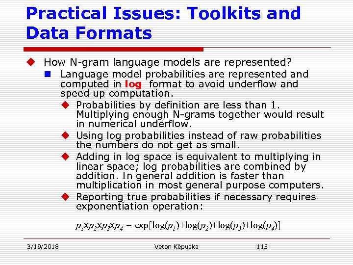 Practical Issues: Toolkits and Data Formats u How N-gram language models are represented? n Language model probabilities are represented and computed in log format to avoid underflow and speed up computation. u Probabilities by definition are less than 1. Multiplying enough N-grams together would result in numerical underflow. u Using log probabilities instead of raw probabilities the numbers do not get as small. u Adding in log space is equivalent to multiplying in linear space; log probabilities are combined by addition. In general addition is faster than multiplication in most general purpose computers. u Reporting true probabilities if necessary requires exponentiation operation: p 1 xp 2 xp 3 xp 4 = exp[log(p 1)+log(p 2)+log(p 3)+log(p 4)] 3/19/2018 Veton Këpuska 115
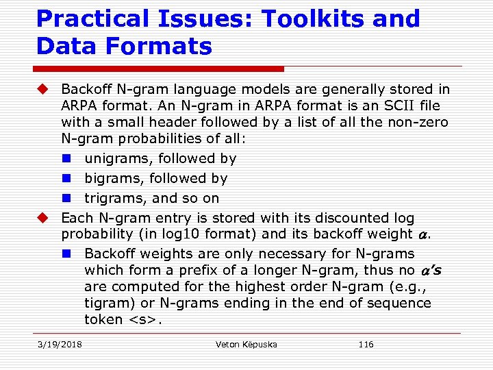 Practical Issues: Toolkits and Data Formats u Backoff N-gram language models are generally stored in ARPA format. An N-gram in ARPA format is an SCII file with a small header followed by a list of all the non-zero N-gram probabilities of all: n unigrams, followed by n bigrams, followed by n trigrams, and so on u Each N-gram entry is stored with its discounted log probability (in log 10 format) and its backoff weight a. n Backoff weights are only necessary for N-grams which form a prefix of a longer N-gram, thus no a’s are computed for the highest order N-gram (e. g. , tigram) or N-grams ending in the end of sequence token
 . 3/19/2018 Veton Këpuska 116
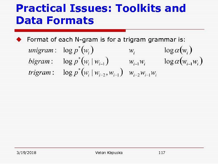 Practical Issues: Toolkits and Data Formats u Format of each N-gram is for a trigrammar is: 3/19/2018 Veton Këpuska 117
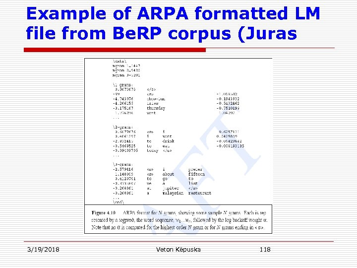 Example of ARPA formatted LM file from Be. RP corpus (Juras 3/19/2018 Veton Këpuska 118
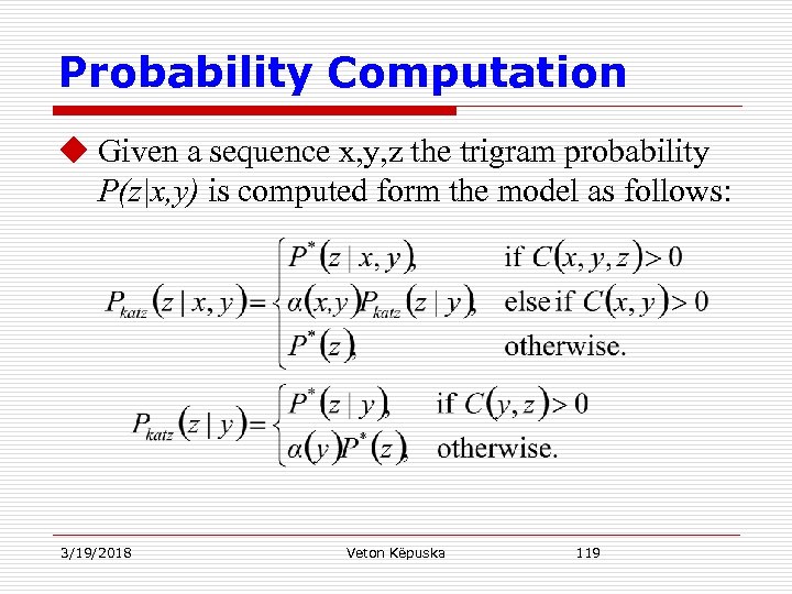 Probability Computation u Given a sequence x, y, z the trigram probability P(z|x, y) is computed form the model as follows: 3/19/2018 Veton Këpuska 119
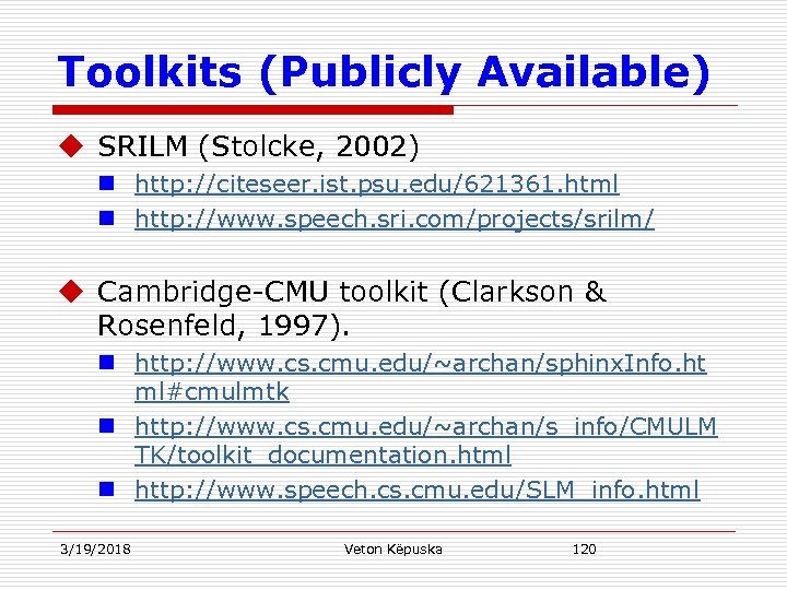 Toolkits (Publicly Available) u SRILM (Stolcke, 2002) n http: //citeseer. ist. psu. edu/621361. html n http: //www. speech. sri. com/projects/srilm/ u Cambridge-CMU toolkit (Clarkson & Rosenfeld, 1997). n http: //www. cs. cmu. edu/~archan/sphinx. Info. ht ml#cmulmtk n http: //www. cs. cmu. edu/~archan/s_info/CMULM TK/toolkit_documentation. html n http: //www. speech. cs. cmu. edu/SLM_info. html 3/19/2018 Veton Këpuska 120
 ADVANCED ISSUES IN LANGUAGE MODELING Advanced Smoothing Methods: Kneser-Ney Smoothing
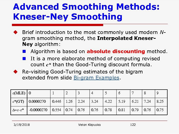 Advanced Smoothing Methods: Kneser-Ney Smoothing u Brief introduction to the most commonly used modern Ngram smoothing method, the Interpolated Kneser. Ney algorithm: n Algorithm is based on absolute discounting method. n It is a more elaborate method of computing revised count c* than the Good-Turing discount formula. u Re-visiting Good-Turing estimates of the bigram extended from slide Bi-gram Examples. c(MLE) 0 1 2 3 4 5 6 7 8 9 c*(GT) 0. 0000270 0. 446 1. 26 2. 24 3. 24 4. 22 5. 19 6. 21 7. 24 8. 25 D=c-c* -0. 0000270 0. 554 0. 76 0. 78 0. 81 0. 79 0. 76 0. 75 3/19/2018 Veton Këpuska 122
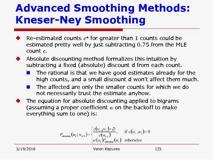 Advanced Smoothing Methods: Kneser-Ney Smoothing u u u Re-estimated counts c* for greater than 1 counts could be estimated pretty well by just subtracting 0. 75 from the MLE count c. Absolute discounting method formalizes this intuition by subtracting a fixed (absolute) discount d from each count. n The rational is that we have good estimates already for the high counts, and a small discount d won’t affect them much. n The affected are only the smaller counts for which we do not necessarily trust the estimate anyhow. The equation for absolute discounting applied to bigrams (assuming a proper coefficient a on the backoff to make everything sum to one) is: 3/19/2018 Veton Këpuska 123
 Advanced Smoothing Methods: Kneser-Ney Smoothing In practice distinct discount values d for the 0 and 1 counts are computed. u Kneser-Neay discounting augments absolute discounting with a more sophisticated way to handle the backoff distribution. Consider the job of predicting the next word in the sentence, assuming we are backing off to a unigram model: n I can’t see without my reading XXXXXX. u The word “glasses” seem much more likely to follow than the word “Francisco”. n But “Francisco” is in fact more common, and thus a unigram model will prefer it to “glasses”. 1. Thus we would like to capture that although “Francisco” is frequent, it is only frequent after the word “San”. 2. The word “glasses” has a much wider distribution. u 3/19/2018 Veton Këpuska 124
 Advanced Smoothing Methods: Kneser-Ney Smoothing u Thus the idea is instead of backing off to the unigram MLE count (the number of times the word w has been seen), we want to use a completely different backoff distribution! n We want a heuristic that more accurately estimates the number of times we might expect to see word w in a new unseen context. n The Kneser-Ney intuition is to base our estimate on the number of different contexts word w has appeared in. n Words that have appeared in more contexts are more likely to appear in some new context as well. n New backoff probability can be expressed as the “continuation probability” presented in following expression: 3/19/2018 Veton Këpuska 125
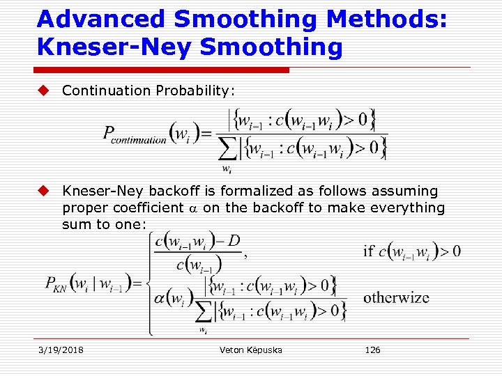 Advanced Smoothing Methods: Kneser-Ney Smoothing u Continuation Probability: u Kneser-Ney backoff is formalized as follows assuming proper coefficient a on the backoff to make everything sum to one: 3/19/2018 Veton Këpuska 126
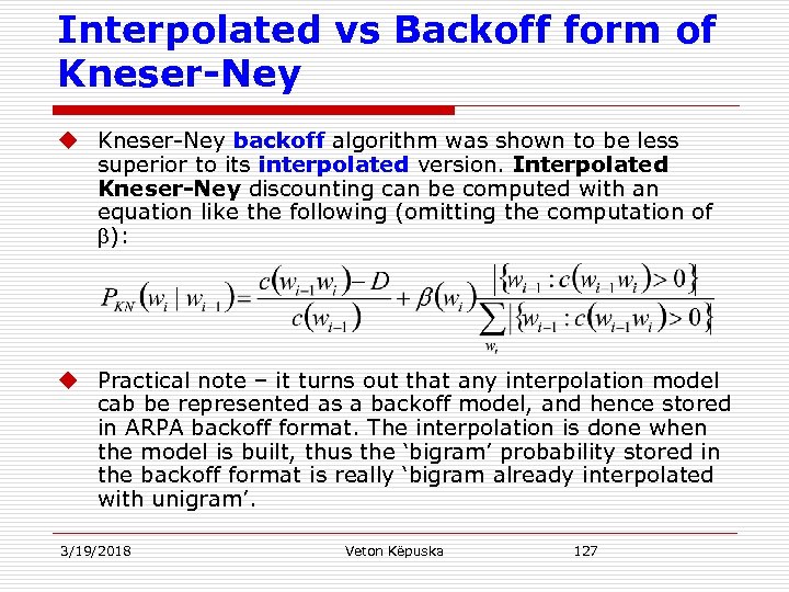 Interpolated vs Backoff form of Kneser-Ney u Kneser-Ney backoff algorithm was shown to be less superior to its interpolated version. Interpolated Kneser-Ney discounting can be computed with an equation like the following (omitting the computation of b): u Practical note – it turns out that any interpolation model cab be represented as a backoff model, and hence stored in ARPA backoff format. The interpolation is done when the model is built, thus the ‘bigram’ probability stored in the backoff format is really ‘bigram already interpolated with unigram’. 3/19/2018 Veton Këpuska 127
 Class-based N-grams or Cluster N -grams
 Class-based N-grams u Class-based N-grams or Cluster N-grams is a variant of the N-gram that uses information about word classes or clusters. It is useful for dealing with scarcity in the training data. u Example: n n 3/19/2018 Suppose for a flight reservation system we want to compute the probability of the bigram to Shanghai, but this bigram never occurs in the training set. Assume that our training data has to London, to Beijing, and to Denver. If we new that these were all cities, and assuming Shanghai does appear in the training set in other contexts, we could predict the likelihood of a city following from. Veton Këpuska 129
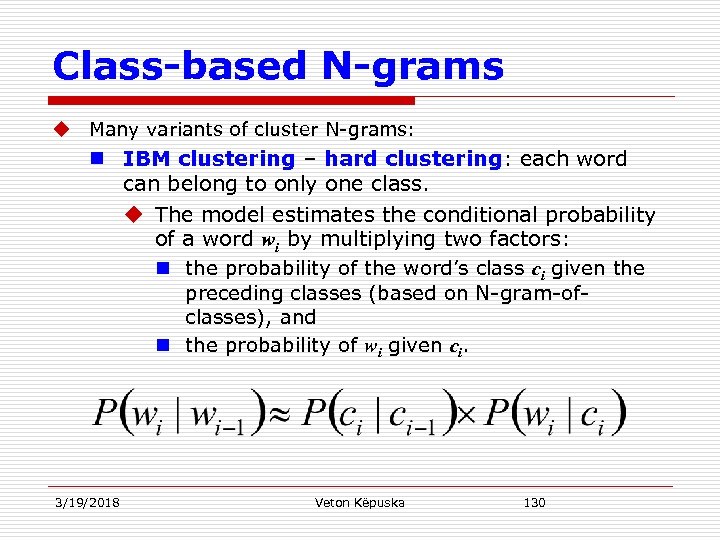 Class-based N-grams u Many variants of cluster N-grams: n IBM clustering – hard clustering: each word can belong to only one class. u The model estimates the conditional probability of a word wi by multiplying two factors: n the probability of the word’s class ci given the preceding classes (based on N-gram-ofclasses), and n the probability of wi given ci. 3/19/2018 Veton Këpuska 130
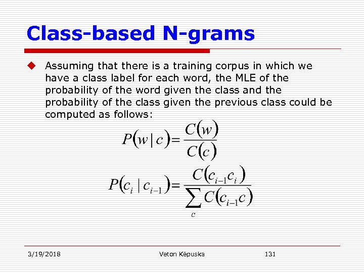 Class-based N-grams u Assuming that there is a training corpus in which we have a class label for each word, the MLE of the probability of the word given the class and the probability of the class given the previous class could be computed as follows: 3/19/2018 Veton Këpuska 131
 Class-based N-grams Cluster N-grams are generally used in two ways: 1. Hand-designed domain-specific word classes. In airline information system we might use classes like: n CITYNAME n AIRLINE n DAYOFWEEK n MONTH, etc. 2. Automatically induce the classes by clustering words in a corpus. n Syntactic categories like part-of-speech tags don’t seem to work well as classes. u Whether automatically induced or hand-designed, cluster N-grams are generally mixed with regular wordbased N-grams. u 3/19/2018 Veton Këpuska 132
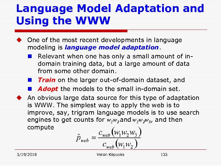 Language Model Adaptation and Using the WWW u One of the most recent developments in language modeling is language model adaptation. n Relevant when one has only a small amount of indomain training data, but a large amount of data from some other domain. n Train on the larger out-of-domain dataset, and n Adopt the models to the small in-domain set. u An obvious large data source for this type of adaptation is WWW. The simplest way to apply the web is to improve, say, trigram language models is to use search engines to get counts for w 1 w 2 and w 1 w 2 w 3, and then compute 3/19/2018 Veton Këpuska 133
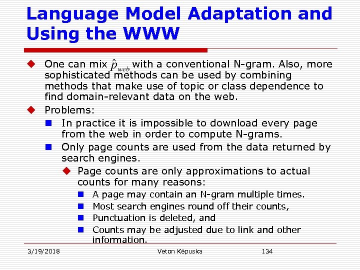 Language Model Adaptation and Using the WWW u One can mix with a conventional N-gram. Also, more sophisticated methods can be used by combining methods that make use of topic or class dependence to find domain-relevant data on the web. u Problems: n In practice it is impossible to download every page from the web in order to compute N-grams. n Only page counts are used from the data returned by search engines. u Page counts are only approximations to actual counts for many reasons: n n 3/19/2018 A page may contain an N-gram multiple times. Most search engines round off their counts, Punctuation is deleted, and Counts may be adjusted due to link and other information. Veton Këpuska 134
 Language Model Adaptation and Using the WWW u The result is not hugely affected in spite of the “noise” due to inaccuracies of the information collected. u It is possible to perform specific adjustments, such as fitting a regression to predict actual word counts from page counts. 3/19/2018 Veton Këpuska 135
 Using Longer Distance Information: A Brief Summary u There are methods for incorporating longer-distance context into N-gram modeling. u While we have limited our discussion mainly to bigram and trigrams, state-of-the-art speech recognition systems, for example, are based on longer distance Ngrams, especially 4 -grams, but also 5 -grams. u Goodman (2006) showed that with 284 million words of training data, 5 -grams do improve perplexity scores over 4 -grams, but not by much. Goodman checked contexts up to 20 -grams, and found that after 6 -grams, longer contexts weren’t useful, at least not with 284 million words of training data. 3/19/2018 Veton Këpuska 136
 More Sophisticated Models u People tend to repeat words they have used before. Thus if a word is used once in a text, it will probably be used again. We can capture this fact by a cache language model (Kuhn and De. Mori, 1990). u To use a unigram cache model to predict word i of a test corpus, we create a unigrammar from the preceding part of the test corpus (words 1 to i− 1), and mix this with our conventional N-gram. We might use only a shorter window from the previous words, rather than the entire set. u Cache language models are very powerful in any applications where we have perfect knowledge of the words. Cache models work less well in domains where the previous words are not known exactly. In speech applications, for example, unless there is some way for users to correct errors, cache models tend to ‘lock-in’ to errors they made on earlier words. 3/19/2018 Veton Këpuska 137
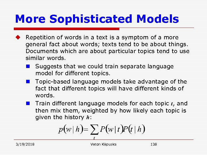 More Sophisticated Models u Repetition of words in a text is a symptom of a more general fact about words; texts tend to be about things. Documents which are about particular topics tend to use similar words. n Suggests that we could train separate language model for different topics. n Topic-based language models take advantage of the fact that different topics will have different kinds of words. n Train different language models for each topic t, and then mix them, weighted by how likely each topic is given the history h: 3/19/2018 Veton Këpuska 138
 More Sophisticated Models u Latent Semantic Indexing: n Based on the intuition that upcoming words are semantically similar to preceding words in the text. n Word similarity is computed from measure of semantic word association such as the latent semantic indexing u Computed from dictionaries or thesauri, then u Mixed with a conventional N-gram. 3/19/2018 Veton Këpuska 139
 More Sophisticated Models u u u Trigger Word based N-grams n Predictor word – called trigger which is not adjacent but is very related: has high mutual information with the word we are trying to predict. Skip N-grams n Preceding context ‘skips over’ some intermediate words such as P(wi|wi-1 wi-2). Variable-length N-grams n Preceding context is extended where a longer phrase is particularly frequent. Using very large and rich contexts can result in very large language models. n These models are often pruned, removing low-probability events. There is a large body of research on integrating sophisticated linguistic structures into language modeling as described in following chapters of the text book. 3/19/2018 Veton Këpuska 140
 ADVACED TOPIC INFORMAITON THEORY BACKGROUND
 Information Theory Background u In previous section, perplexity was introduced as a way to evaluate N-gram models on a test set. n A better N-gram model is one which assigns a higher probability to the test data n Perplexity is a normalized version of the probability of the test set. u Another way to think about perplexity is based on the information-theoretic concept of cross-entropy. u This section introduces fundamentals of information theory including the concept of cross-entropy. n Reference: “Elements of Information Theory”, Cover and Thomas. Wiley-Interscience, 1991 3/19/2018 Veton Këpuska 142
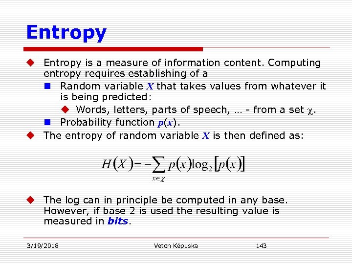 Entropy u Entropy is a measure of information content. Computing entropy requires establishing of a n Random variable X that takes values from whatever it is being predicted: u Words, letters, parts of speech, … - from a set c. n Probability function p(x). u The entropy of random variable X is then defined as: u The log can in principle be computed in any base. However, if base 2 is used the resulting value is measured in bits. 3/19/2018 Veton Këpuska 143
 Entropy u The most intuitive way to define entropy for computer scientist is to think of the entropy as a lower bound on the number of bits it would take to encode a certain decision or piece of information in the optimal coding scheme. u In Cover and Thomas the following example is provided: n Imagine that we want to place a bet on a horse race but it is too far to go all the way to Yonkers Racetrack, and we’d like to send a short message to the bookie to tell him which horse to bet on. n Suppose there are eight horses in this particular race. One way to encode this message is just to use the binary representation of the horse’s number as the code; thus horse 1 would be 001, horse 2 - 010, horse 3 - 011, and so on, with horse 8 coded as 000. If we spend the whole day betting, and each horse is coded with 3 bits, on the average we would be sending 3 bits per race. n Can we do better? 3/19/2018 Veton Këpuska 144
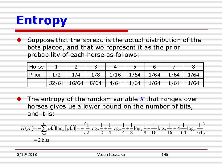 Entropy u Suppose that the spread is the actual distribution of the bets placed, and that we represent it as the prior probability of each horse as follows: Horse 1 2 3 4 5 6 7 8 Prior 1/2 1/4 1/8 1/16 1/64 8/64 4/64 1/64 32/64 16/64 u The entropy of the random variable X that ranges over horses gives us a lower bound on the number of bits, and it is: 3/19/2018 Veton Këpuska 145
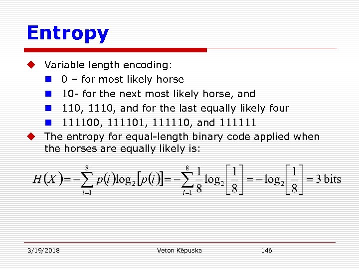 Entropy u Variable length encoding: n 0 – for most likely horse n 10 - for the next most likely horse, and n 110, 1110, and for the last equally likely four n 111100, 111101, 111110, and 111111 u The entropy for equal-length binary code applied when the horses are equally likely is: 3/19/2018 Veton Këpuska 146
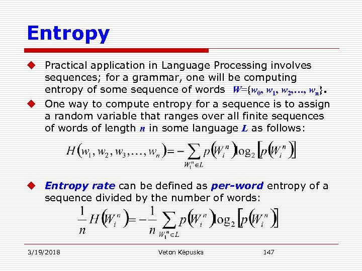 Entropy u Practical application in Language Processing involves sequences; for a grammar, one will be computing entropy of some sequence of words W={w 0, w 1, w 2, …, wn}. u One way to compute entropy for a sequence is to assign a random variable that ranges over all finite sequences of words of length n in some language L as follows: u Entropy rate can be defined as per-word entropy of a sequence divided by the number of words: 3/19/2018 Veton Këpuska 147
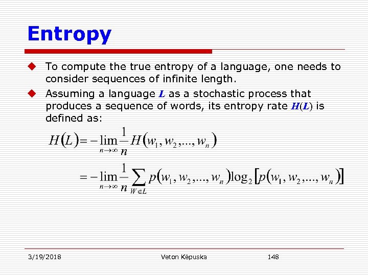 Entropy u To compute the true entropy of a language, one needs to consider sequences of infinite length. u Assuming a language L as a stochastic process that produces a sequence of words, its entropy rate H(L) is defined as: 3/19/2018 Veton Këpuska 148
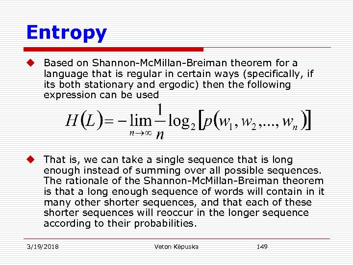 Entropy u Based on Shannon-Mc. Millan-Breiman theorem for a language that is regular in certain ways (specifically, if its both stationary and ergodic) then the following expression can be used u That is, we can take a single sequence that is long enough instead of summing over all possible sequences. The rationale of the Shannon-Mc. Millan-Breiman theorem is that a long enough sequence of words will contain in it many other shorter sequences, and that each of these shorter sequences will reoccur in the longer sequence according to their probabilities. 3/19/2018 Veton Këpuska 149
 Entropy u A stochastic process is said to be stationary if the probabilities it assigns to a sequence are invariant with respect to shifts in the time index. n The probability distribution for words at time t, is the same as the probability distribution at time t+1. n Markov models and hence N-grams are stationary. u In bigram Pi is dependent only on Pi-1. So if we shift our time index by x, Pi+x is still dependent on Pi+x-1. u However, natural language is not stationary, since as we will see in latter (Ch 12 of the book) the probability of upcoming words can be dependent on events that were arbitrarily distant in time and thus time dependent. u Consequently, statistical models only give an approximation to the correct distributions and entropies of natural language. 3/19/2018 Veton Këpuska 150
 Entropy u To summarize: n By making some incorrect but convenient simplifying n assumptions, we can compute the entropy of some stochastic process by taking a very long sample of the output, and computing its average log probability. In the next section we talk about the why and how; u why we would want to do this (i. e. , for what kinds of problems would the entropy tell us something useful), and u how to compute the probability of a very long sequence. 3/19/2018 Veton Këpuska 151
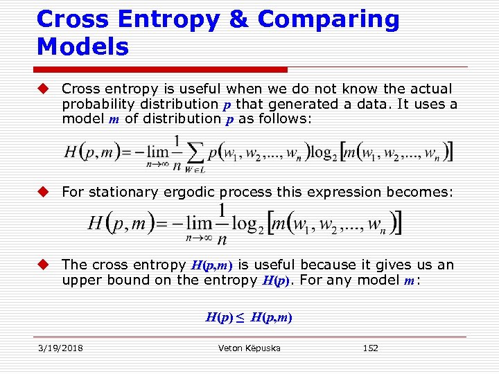 Cross Entropy & Comparing Models u Cross entropy is useful when we do not know the actual probability distribution p that generated a data. It uses a model m of distribution p as follows: u For stationary ergodic process this expression becomes: u The cross entropy H(p, m) is useful because it gives us an upper bound on the entropy H(p). For any model m: H(p) ≤ H(p, m) 3/19/2018 Veton Këpuska 152
 Cross Entropy & Comparing Models u This means that we can use some simplified model m to help estimate the true entropy of a sequence of symbols drawn according to probability p. n The more accurate m is, the closer the cross entropy H(p, m) will be to the true entropy H(p). n Thus the difference between H(p, m) and H(p) is a measure of how accurate a model is. n Between two models m 1 and m 2, the more accurate model will be the one with the lower cross-entropy. (The cross-entropy can never be lower than the true entropy, so a model cannot err by underestimating the true entropy). 3/19/2018 Veton Këpuska 153
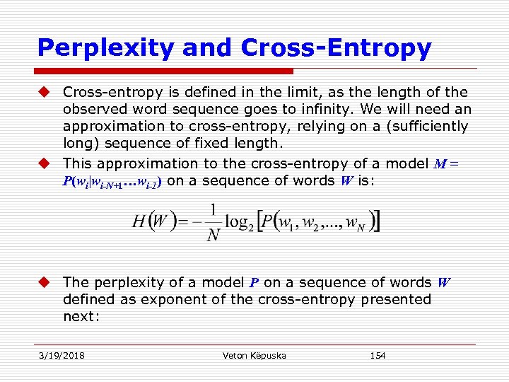 Perplexity and Cross-Entropy u Cross-entropy is defined in the limit, as the length of the observed word sequence goes to infinity. We will need an approximation to cross-entropy, relying on a (sufficiently long) sequence of fixed length. u This approximation to the cross-entropy of a model M = P(wi|wi-N+1…wi-1) on a sequence of words W is: u The perplexity of a model P on a sequence of words W defined as exponent of the cross-entropy presented next: 3/19/2018 Veton Këpuska 154
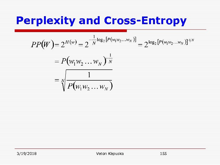 Perplexity and Cross-Entropy 3/19/2018 Veton Këpuska 155
 Advanced Topic The Entropy of English and Entropy Rate Constancy
 The Entropy of English and Entropy Rate Constancy u As we suggested in the previous section, the cross-entropy of some model m can be used as an upper bound on the true entropy of some process. We can use this method to get an estimate of the true entropy of English. n Why should we care about the entropy of English? 1. Knowing the entropy of English would give us a solid lower bound for all of our future experiments on probabilistic grammars. We can use the entropy of English to help understand what parts of a language provide the most information: u Is the predictability of English mainly based on u Word order u Semantics, u Morphology, u Consistency, or on u Pragmatic cues? u Answering this question can help us immensely in knowing where to focus our language-modeling efforts. 2. 3/19/2018 Veton Këpuska 157
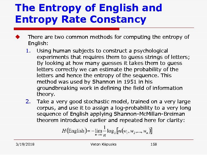 The Entropy of English and Entropy Rate Constancy u There are two common methods for computing the entropy of English: 1. Using human subjects to construct a psychological experiments that requires them to guess strings of letters; By looking at how many guesses it takes them to guess letters correctly we can estimate the probability of the letters and hence the entropy of the sequence. This method was used by Shannon in 1951 in his groundbreaking work in defining the field of information theory. 2. Take a very good stochastic model, trained on a very large corpus, and use it to assign a log-probability to a very long sequence of English applying Shannon-Mc. Millan-Breiman theorem introduced earlier and repeated here for clarity: 3/19/2018 Veton Këpuska 158
 Shannon Experiment The actual experiment is designed as follows: u We present a subject with some English text and ask the subject to guess the next letter. u The subjects will use their knowledge of the language to guess the most probable letter first, the next most probable next, and so on. u We record the number of guesses it takes for the subject to guess correctly. u u Shannon’s insight was that the entropy of the number-of-guesses sequence is the same as the entropy of English. (The intuition is that given the number-ofguesses sequence, we could reconstruct the original text by choosing the “nth most probable” letter whenever the subject took n guesses). This methodology requires the use of letter guesses rather than word guesses (since the subject sometimes has to do an exhaustive search of all the possible letters!), and so Shannon computed the per-letter entropy of English rather than the per-word entropy. He reported an entropy of 1. 3 bits (for 27 characters (26 letters plus space)). Shannon’s estimate is likely to be too low, since it is based on a single text (Jefferson the Virginian by Dumas Malone). Shannon notes that his subjects had worse guesses (hence higher entropies) on other texts (newspaper writing, scientific work, and poetry). More recently variations on the Shannon experiments include the use of a gambling paradigm where the subjects get to bet on the next letter (Cover and King, 1978; Cover and Thomas, 1991). 3/19/2018 Veton Këpuska 159
 Computer Based Computation of Entropy of English u u u The second method for computing the entropy of English helps avoid the single text problem that confounds Shannon’s results. For example, Brown et al. (1992 a) trained a trigram language model on 583 million words of English, (293, 181 different types) and used it to compute the probability of the entire Brown corpus (1, 014, 312 tokens). The training data include newspapers, encyclopedias, novels, office correspondence, proceedings of the Canadian parliament, and other miscellaneous sources. They then computed the character-entropy of the Brown corpus, by using their word-trigrammar to assign probabilities to the Brown corpus, considered as a sequence of individual letters. They obtained an entropy of 1. 75 bits per character (where the set of characters included all the 95 printable ASCII characters). 3/19/2018 Veton Këpuska 160
 Computer Based Computation of Entropy of English u The average length of English written words (including space) has been reported at 5. 5 letters (N´adas, 1984). u If this is correct, it means that the Shannon estimate of 1. 3 bits per letter corresponds to a per-word perplexity of 142 for general English. u The numbers we report earlier for the WSJ experiments are significantly lower than this, since the training and test set came from the same sub-sample of English. That is, those experiments underestimate the complexity of English (since the Wall Street Journal looks very little like Shakespeare, for example). 3/19/2018 Veton Këpuska 161
 Constant Information/Entropy Rate of Speech u A number of scholars have independently made the intriguing suggestion that entropy rate plays a role in human communication in general (Lindblom, 1990; Van Son et al. , 1998; Aylett, 1999; Genzel and Charniak, 2002; Van Son and Pols, 2003). u Constant information/entropy rate of speech: n n 3/19/2018 The idea is that people speak so as to keep the rate of information being transmitted per second roughly constant, i. e. transmitting a constant number of bits per second, or maintaining a constant entropy rate. Since the most efficient way of transmitting information through a channel is at a constant rate, language may even have evolved for such communicative efficiency (Plotkin and Nowak, 2000). There is a wide variety of evidence for the constant entropy rate hypothesis. One class of evidence, for speech, shows that speakers shorten predictable words (i. e. they take less time to say predictable words) and lengthen unpredictable words (Aylett, 1999; Jurafsky et al. , 2001; Aylett and Turk, 2004). Veton Këpuska 162
 Constant Information/Entropy Rate of Speech u In another line of research, Genzel and Charniak (2002, 2003) show that entropy rate constancy makes predictions about the entropy of individual sentences from a text. n In particular, they show that it predicts that local measures of sentence entropy which ignore previous discourse context (for example the N-gram probability of sentence), should increase with the sentence number, and they document this increase in corpora. n Keller (2004) provides evidence that entropy rate plays a role for the addressee as well, showing a correlation between the entropy of a sentence and the processing effort it causes in comprehension, as measured by reading times in eye-tracking data. 3/19/2018 Veton Këpuska 163
 END
END


