SAMPLE SELECTION in Earnings Equation Cheti Nicoletti ISER

SAMPLE SELECTION in Earnings Equation Cheti Nicoletti ISER, University of Essex

Wage equation and labour participation for women Gourieroux C. (2000), Econometrics of Qualitative Dependent Variables, Cambridge University Press, Cambridge • Let y* be the potential offered wage and let w be the reservation wage then the observed wage y is given by • Let us consider the following very simple earnings profile equation

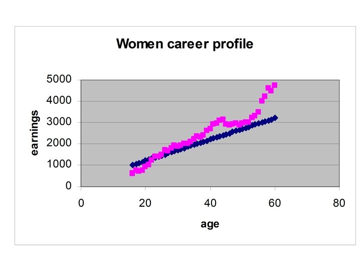
Women in the labour force are not a random sample • “Women’s labour force participation rates are highly dependent on age. ” Gourieroux (2000) • Labour participation is in general lower for women aged: – 16 -20 because some women are still studying – 25 -44 for work interruption linked to children – 55 -60 because some women prefer to retire early • Presumably the earnings observed for women aged – 16 -20 are lower than if all women worked – 25 -44 are higher because women with higher earnings are less incline to work interruptions – 55 -60 are higher because women with higher earnings are less incline to retire early

Sample selection model Labour participation equation • Probit model for labour participation

Joint model for the log-earnings and the labour participation equations Generalized TOBIT MODEL • Possible candidates for x: education dummies, age, work experience • Possible candidates for z: age, education, number of children, dummies for the presence of children <5, for cohabiting, for widow, regional unemployment rate.

Sample selection problem E(y*|d=1, x, z)=x +E( |d=1, x, z)= E( |ν>-zδ )= E(y*|d=1, x, z)= X

Two-step estimation • 1 STEP: estimation of a probit model for the probability to be in the labour market, Π Pr(di=1|zi)di Pr(di=0|zi)1 -di=Π (zi ) di (-zi ) 1 -di • 2 STEP: estimation of the regression model with an additional variable (the inverse Mill’s ratio) using the subsample of individuals with di=1 (and using some IV restrictions)

Testing selectivity • • • If the error terms and u are uncorrelated, then the selection problem is ignorable. H 0: σ u =0 Verifying H 0 is equivalent to verify whether the coefficient of the additional variable in the equation is zero (using for ex. a Wald test) Notice that the errors are heteroskedastic so a proper estimation should be adopted to estimate the standard errors

Generalized Tobit: Maximum Likelihood Estimation

heckman • The heckman command is used to estimate Generalized Tobit or Tobit of the 2 nd type using ML estimation (default option) or the two -step estimation (option [twostep]) heckman y x 1 x 2 … xk, select(z 1 z 2 … zs) heckman y x 1 x 2 … xk, select(d = z 1 z 2 … zs) heckman y x 1 x 2 … xk, select(z 1 z 2 … zs) twostep

Generalized Tobit: Maximum Likelihood Estimation

Joint model for log-earnings and response probability • Possible candidates for x: education dummies, age, work experience • d* is the propensity to respond to the earnings question • Z: mode of interview, education, gender, age, etc.

Item nonresponse for income equation or poverty model in cross section sample surveys: Potential explanatory variables: • Socio-demographic variables: age, gender, level of education, number of adults, number of children. • Situational economic circumstance: labour status activity. • Data collection characteristics: mode of the interview, number of visits, duration of the interview. (These are plausible IV)

Attrition in panel surveys has two possible causes: failed contact and refusal The potential variables explaining attrition (contact and cooperation) are lagged variables observed in the last wave. The equation of interest has to use lagged variables (otherwise we have missing explanatory variables too) • Socio-demographic variables: age, gender, level of education, number of adults, number of children. • Social-integration: talking often to neighbours, cohabitation, house ownership. • Situational economic circumstance: labour status activity, household equalised income. • Data collection characteristics: mode of the interview, number of visits, duration of the interview, same interviewer across wave, duration of the panel, length of the fieldwork. (These are plausible IV)

How to use weights in Stata • Most Stata commands can deal with weighted data. Stata allows four kinds of weights: 1. fweights, or frequency weights, are weights that indicate the number of duplicated observations. 2. pweights, or sampling weights, are weights that denote the inverse of the probability that the observation is included due to the sampling design, nonresponse or sample selection. 3. aweights, or analytic weights, are weights that are inversely proportional to the variance of an observation; i. e. , the variance of the j-th observation is assumed to be sigma^2/w_j, where w_j are the weights. 4. iweights, or importance weights, are weights that indicate the "importance" of the observation in some vague sense.

Option pweights • Usually sample surveys provide weights to take account of sampling design, nonresponse. • Let p be individual weight • Then we can run a regression with weighted observations regress y x 1 x 2 … xk [pweight=p] • Let us assume to have a random sample affected by nonresponse, but weights to take account of unit nonresponse are not available • A possible way to estimate your own weights is described in the following: probit d z 1 z 2 … zs predict prop gen invprop=1/prop reg y x 1 x 2 … xk [pweight=invprop]

For complex survey design it is better to use • svyset [pweight=p] • svy: regress y x 1 x 2 … xk • svyset have options for cluster sampling designs or other complex design • To declare survey design with stratum • svyset [pweight=p], strata(stratid)

Stata propensity score methods for evaluation of treatment Abadie A. , Drukker D. , Herr J. L. , Imbens G. W. (2001), Implementing Matching Estimators for Average Treatment Effects in Stata, The Stata Journal, 1, 1 -18 http: //ksghome. harvard. edu/~. aabadie. academic. ksg/software. html Becker S. O. , Ichino A. (2002), Estimation of average treatment effects based on propensity scores. The Stata Journal, 2, 358377 http: //www. lrz-muenchen. de/~sobecker/pscore. html Sianesi B. (2001), Implementing Propensity Score Matching Estimators with STATA, UK Stata Users Group, VII Meeting London, http: //ideas. repec. org/c/bocode/s 432001. html