Risk and Return Part 2 For 9

Risk and Return – Part 2 For 9. 220, Term 1, 2002/03 02_Lecture 13. ppt Instructor Version

Outline 1. 2. Introduction Looking forward o 3. Portfolios o o 4. 5. Ex ante expectation, standard deviation, correlation coefficient, and covariance of returns Portfolio weights Short selling Expected returns Standard deviation of returns Domination Summary and Conclusions

Introduction o o o We have seen there is risk in financial markets. Investors seek to reduce risk by investing in portfolios of securities. We shall learn how to determine the expected returns and riskiness of portfolios and we will see the benefits of diversification. Since investors are risk-averse, we introduce the concept of domination to help eliminate portfolios that investors would not consider.

Looking Forward o o In our previous analysis of security return and risk measures, we looked at past or historical data to calculate mean returns and sample standard deviations of returns. Now we will also look forward and use our expectations of future events to make estimates of expected returns, standard deviations.

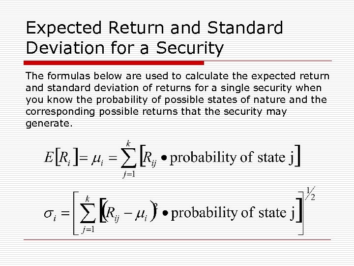Expected Return and Standard Deviation for a Security The formulas below are used to calculate the expected return and standard deviation of returns for a single security when you know the probability of possible states of nature and the corresponding possible returns that the security may generate.

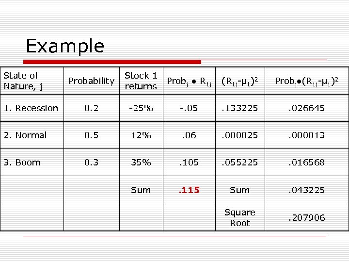Example State of Nature, j Probability Stock 1 returns Probj ● R 1 j (R 1 j-μ 1)2 Probj●(R 1 j-μ 1)2 1. Recession 0. 2 -25% -. 05 . 133225 . 026645 2. Normal 0. 5 12% . 06 . 000025 . 000013 3. Boom 0. 3 35% . 105 . 055225 . 016568 Sum . 115 Sum . 043225 Square Root . 207906

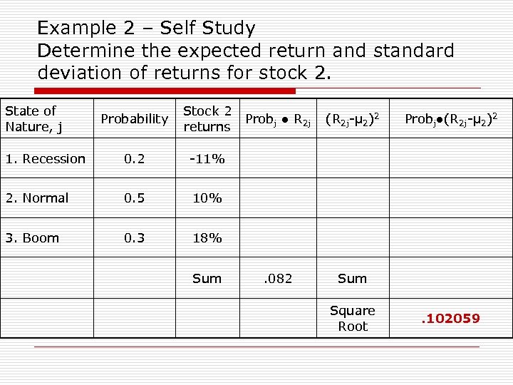Example 2 – Self Study Determine the expected return and standard deviation of returns for stock 2. State of Nature, j Probability Stock 2 returns 1. Recession 0. 2 -11% 2. Normal 0. 5 10% 3. Boom 0. 3 18% Sum Probj ● R 2 j (R 2 j-μ 2)2 . 082 Sum Square Root Probj●(R 2 j-μ 2)2 . 102059

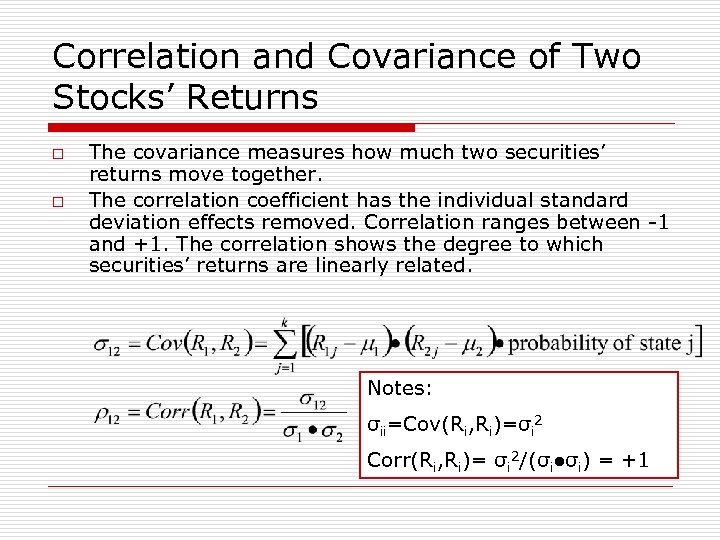Correlation and Covariance of Two Stocks’ Returns o o The covariance measures how much two securities’ returns move together. The correlation coefficient has the individual standard deviation effects removed. Correlation ranges between -1 and +1. The correlation shows the degree to which securities’ returns are linearly related. Notes: σii=Cov(Ri, Ri)=σi 2 Corr(Ri, Ri)= σi 2/(σi●σi) = +1

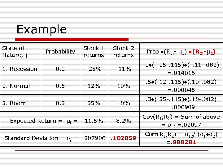Example State of Nature, j 1. Recession Probability 0. 2 Stock 1 returns -25% Stock 2 returns Probj●(R 1 j- μ 1) ●(R 2 j-μ 2) -11% . 2●(-. 25 -. 115)●(-. 11 -. 082) =. 014016 2. Normal 0. 5 12% 10% . 5●(. 12 -. 115)●(. 10 -. 082) =. 000045 3. Boom 0. 3 35% 18% . 3●(. 35 -. 115)●(. 18 -. 082) =. 006909 8. 2% Cov(R 1, R 2) = Sum of above = σ12 =. 02097 Expected Return = μi = 11. 5% Standard Deviation = σi =. 207906. 102059 Corr(R 1, R 2) = σ12/ (σ1●σ2) =. 988281

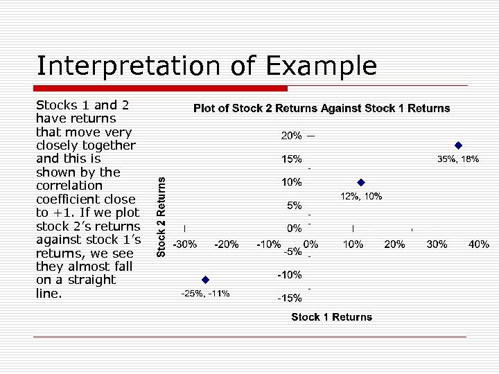Interpretation of Example Stocks 1 and 2 have returns that move very closely together and this is shown by the correlation coefficient close to +1. If we plot stock 2’s returns against stock 1’s returns, we see they almost fall on a straight line.

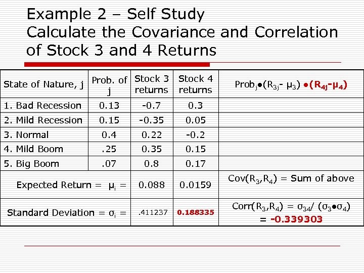Example 2 – Self Study Calculate the Covariance and Correlation of Stock 3 and 4 Returns Stock 3 State of Nature, j Prob. of returns j Stock 4 returns 1. Bad Recession 0. 13 -0. 7 0. 3 2. Mild Recession 0. 15 -0. 35 0. 05 3. Normal 0. 4 0. 22 -0. 2 4. Mild Boom . 25 0. 35 0. 15 5. Big Boom . 07 0. 8 Probj●(R 3 j- μ 3) ●(R 4 j-μ 4) 0. 17 Expected Return = μi = Standard Deviation = σi = 0. 088 0. 0159 . 411237 0. 188335 Cov(R 3, R 4) = Sum of above Corr(R 3, R 4) = σ34/ (σ3●σ4) = -0. 339303

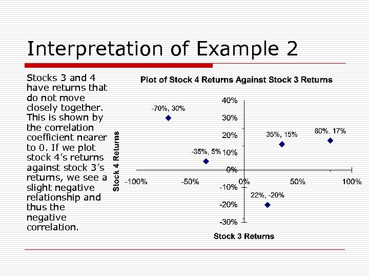Interpretation of Example 2 Stocks 3 and 4 have returns that do not move closely together. This is shown by the correlation coefficient nearer to 0. If we plot stock 4’s returns against stock 3’s returns, we see a slight negative relationship and thus the negative correlation.

Portfolios o Definition: A portfolio is the collection of securities that comprise an individuals investments. n A portfolio may be composed of subportfolios. E. g. , An investor may hold a portfolio of stocks, a portfolio of bonds, and a real estate portfolio. The three portfolios combined are the portfolio of the investments held by the individual.

Portfolio Weights o o The weight of a security in a portfolio at a particular point in time is equal to the security’s market value divided by the total value of the portfolio. Determine the weights for the portfolio that consists of the following: n n n $3, 000 of IBM stock $200 of Nortel stock $10, 000 of T-bills $800 of TD’s Canadian Index Mutual Fund $6, 000 of Gov’t of Canada 30 -year bonds

Negative Portfolio Weights? … Borrowing o o If you borrow money to purchase securities for your portfolio, the securities’ values add in as positive amounts to the market value of the portfolio, but the borrowed money comes in as a negative amount for the market value of the portfolio. Calculate the portfolio weights for the following: n Borrowed $5, 000 to help buy the following securities: o $3, 000 Nova Corp. Stock o $4, 000 BCE Stock o $500 Stelco Stock

Negative Portfolio Weights? … Short Selling o A short sale occurs when you sell something you do not have. n Process for the short sale of a stock o o n To exit the short position, you must o o Borrow the stock (from your broker) Sell the stock Repurchase the stock Return it to your broker (from whom you borrowed the stock) When a short sale exists within a portfolio, the market value of the short security comes into the portfolio as a negative amount. Calculate the portfolio weights given the following: n n n Own 100 shares of Microsoft, market price is $80/share Short 1, 000 shares of Nortel, market price is $2/share Own 100 shares of GM, market price is $40/share

Short selling and borrowing – actually very similar! o o Short selling and borrowing are really very similar. Consider borrowing $961. 54 @ 5% for one year. In one year’s time, $1, 000 must be repaid. n Now consider short selling a T-bill that matures in 1 year and yields 5% (effective annual rate). The proceeds from the short sale will be the current market price of the T-bill and that is $961. 54. n When the short position is exited in one year (just as the T-bill is maturing), $1, 000 must be repaid to repurchase the T-bill so that the T-bill can be returned to the broker. The cash-flow effects of borrowing the money or shorting the T-bill are basically the same! Hence it is not surprising they are treated in the same way when determining portfolio values and weights.

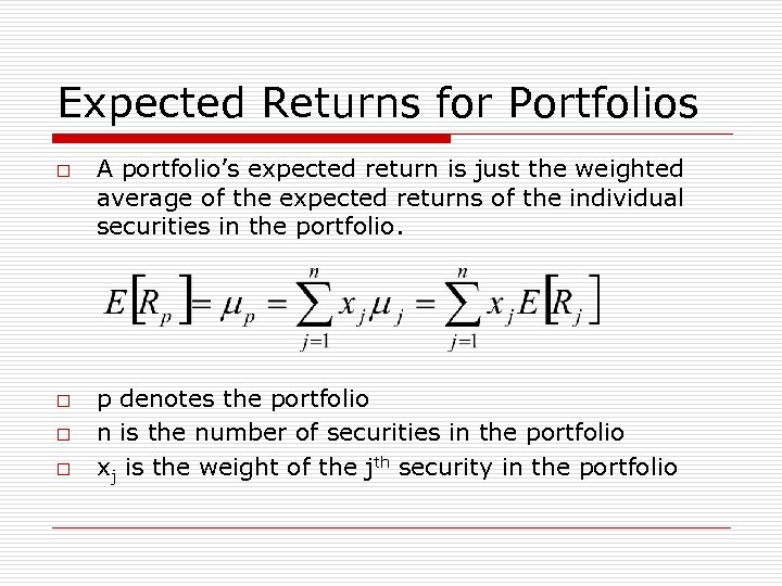Expected Returns for Portfolios o o A portfolio’s expected return is just the weighted average of the expected returns of the individual securities in the portfolio. p denotes the portfolio n is the number of securities in the portfolio xj is the weight of the jth security in the portfolio

Example # Security E[Rj] Securities j Owned Current Market Price Per Market Value Security Portfolio Weight E[Rj]●xj 1 15% 400 $25. 00 $10, 000. 00 0. 1 0. 015 2 18% 500 $30. 00 $15, 000. 00 0. 15 0. 027 3 22% 600 $12. 00 $7, 200. 00 0. 072 0. 01584 4 25% 530 $10. 00 $5, 300. 00 0. 053 0. 01325 5 4% 50 $1, 000. 00 $50, 000. 00 0. 5 0. 02 6 6% 500 $25. 00 $12, 500. 00 0. 125 0. 0075 Sum $100, 000. 00 1 9. 859%

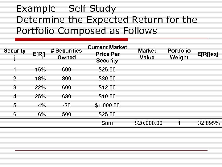Example – Self Study Determine the Expected Return for the Portfolio Composed as Follows E[Rj] # Securities Owned Current Market Price Per Security 1 15% 600 $25. 00 2 18% 300 $30. 00 3 22% 600 $12. 00 4 25% 630 $10. 00 5 4% -30 $1, 000. 00 6 6% 500 $25. 00 Sum Security j Market Value Portfolio Weight E[Rj]●xj $20, 000. 00 1 32. 895%

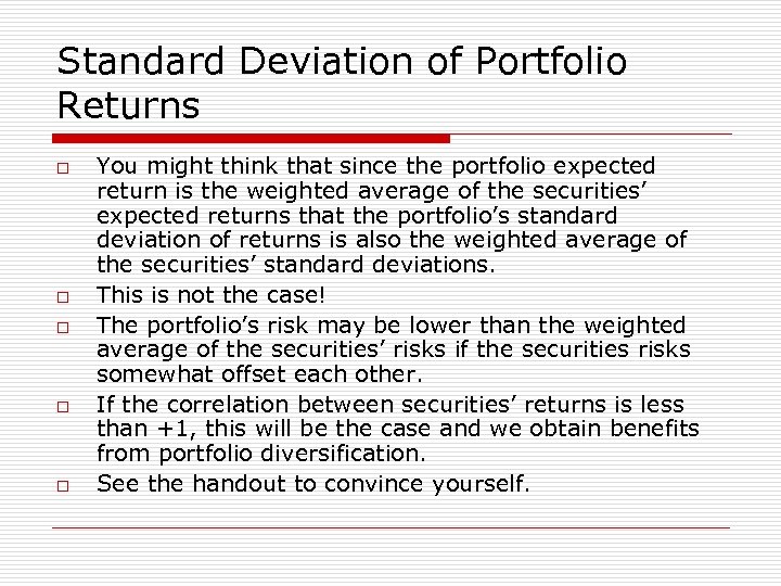Standard Deviation of Portfolio Returns o o o You might think that since the portfolio expected return is the weighted average of the securities’ expected returns that the portfolio’s standard deviation of returns is also the weighted average of the securities’ standard deviations. This is not the case! The portfolio’s risk may be lower than the weighted average of the securities’ risks if the securities risks somewhat offset each other. If the correlation between securities’ returns is less than +1, this will be the case and we obtain benefits from portfolio diversification. See the handout to convince yourself.

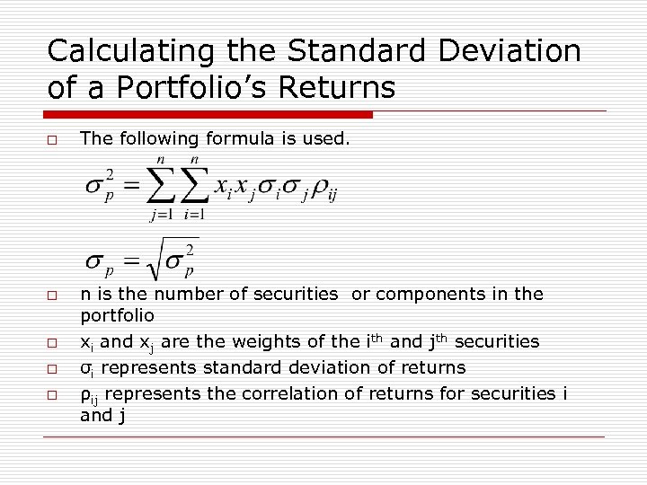Calculating the Standard Deviation of a Portfolio’s Returns o o o The following formula is used. n is the number of securities or components in the portfolio xi and xj are the weights of the ith and jth securities σi represents standard deviation of returns ρij represents the correlation of returns for securities i and j

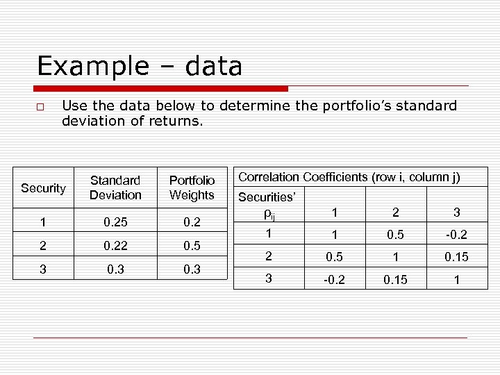Example – data o Use the data below to determine the portfolio’s standard deviation of returns. Security Standard Deviation Portfolio Weights 1 0. 25 0. 2 2 0. 22 0. 5 3 0. 3 Correlation Coefficients (row i, column j) Securities’ ρij 1 2 3 1 1 0. 5 -0. 2 2 0. 5 1 0. 15 3 -0. 2 0. 15 1

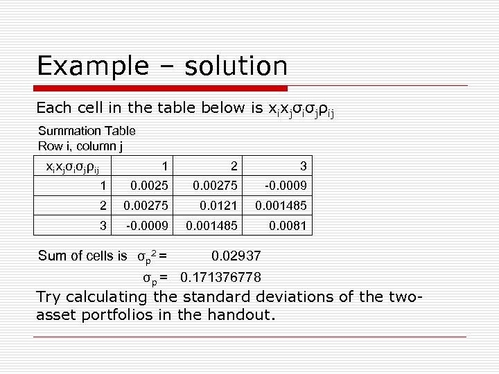Example – solution Each cell in the table below is xixjσiσjρij Summation Table Row i, column j xixjσiσjρij 1 2 3 1 0. 0025 0. 00275 -0. 0009 2 0. 00275 0. 0121 0. 001485 3 -0. 0009 0. 001485 0. 0081 Sum of cells is σp 2 = 0. 02937 σp = 0. 171376778 Try calculating the standard deviations of the twoasset portfolios in the handout.

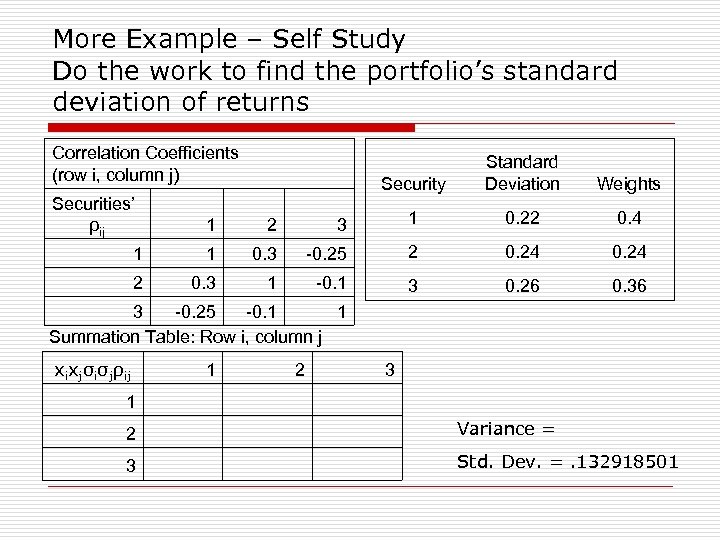More Example – Self Study Do the work to find the portfolio’s standard deviation of returns Correlation Coefficients (row i, column j) Security Standard Deviation Weights Securities’ ρij 1 2 3 1 0. 22 0. 4 1 1 0. 3 -0. 25 2 0. 24 2 0. 3 1 -0. 1 3 0. 26 0. 36 3 -0. 25 -0. 1 1 Summation Table: Row i, column j xixjσiσjρij 1 2 3 1 2 Variance = 3 Std. Dev. =. 132918501

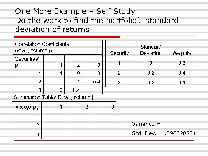One More Example – Self Study Do the work to find the portfolio’s standard deviation of returns Correlation Coefficients (row i, column j) Security Standard Deviation Weights Securities’ ρij 1 2 3 1 0 0. 5 1 1 0 0 2 0. 4 2 0 1 0. 4 3 0. 1 3 0 0. 4 1 Summation Table: Row i, column j xixjσiσjρij 1 2 3 1 2 Variance = 3 Std. Dev. =. 096020831

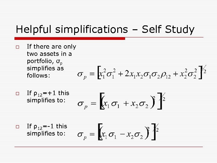Helpful simplifications – Self Study o o o If there are only two assets in a portfolio, σp simplifies as follows: If ρ12=+1 this simplifies to: If ρ12=-1 this simplifies to:

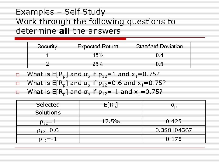Examples – Self Study Work through the following questions to determine all the answers Security o 15% 0. 4 2 o Standard Deviation 1 o Expected Return 25% 0. 5 What is E[Rp] and σp if ρ12=1 and x 1=0. 75? What is E[Rp] and σp if ρ12=0. 6 and x 1=0. 75? What is E[Rp] and σp if ρ12=-1 and x 1=0. 75? Selected Solutions E[Rp] σp ρ12=1 17. 5% 0. 425 ρ12=0. 6 0. 388104367 ρ12=-1 0. 175

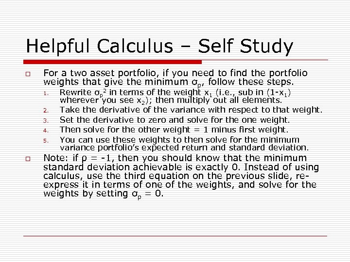Helpful Calculus – Self Study o For a two asset portfolio, if you need to find the portfolio weights that give the minimum σp, follow these steps. 1. 2. 3. 4. 5. o Rewrite σp 2 in terms of the weight x 1 (i. e. , sub in (1 -x 1) wherever you see x 2); then multiply out all elements. Take the derivative of the variance with respect to that weight. Set the derivative to zero and solve for the one weight. Then solve for the other weight = 1 minus first weight. You can use these weights to then solve for the minimum variance portfolio’s expected return and standard deviation. Note: if ρ = -1, then you should know that the minimum standard deviation achievable is exactly 0. Instead of using calculus, use third equation on the previous slide, reexpress it in terms of one of the weights, and solve for the weights by setting σp = 0.

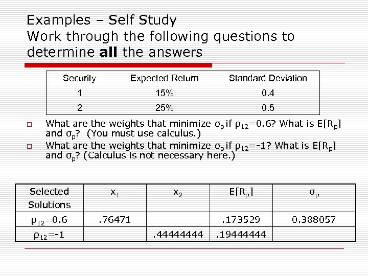Examples – Self Study Work through the following questions to determine all the answers Security 15% 0. 4 2 o Standard Deviation 1 o Expected Return 25% 0. 5 What are the weights that minimize σp if ρ12=0. 6? What is E[Rp] and σp? (You must use calculus. ) What are the weights that minimize σp if ρ12=-1? What is E[Rp] and σp? (Calculus is not necessary here. ) Selected Solutions x 1 ρ12=0. 6 . 76471 ρ12=-1 x 2 σp . 173529. 4444 E[Rp] 0. 388057 . 19444444

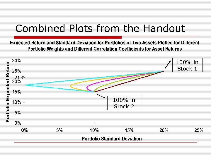Combined Plots from the Handout 100% in Stock 1 21% 100% in Stock 2

Domination o o Investors are assumed to be risk averse. n Prefer a lower risk for a given level of expected return. n Prefer a higher expected return for a given level of risk. We say a portfolio is dominated if, given risk aversion, we can immediately conclude an investor will not consider it. n I. e. , it is dominated if another portfolio exists that has at least as high expected return but lower risk n Or, it is dominated if another portfolio exists that has the no greater risk, but a higher expected return.

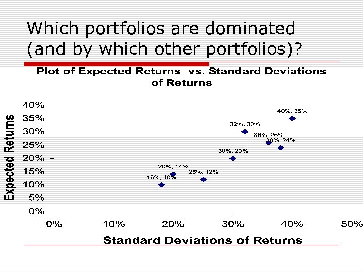Which portfolios are dominated (and by which other portfolios)?

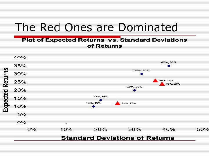The Red Ones are Dominated

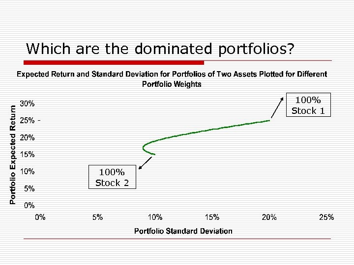Which are the dominated portfolios? 100% Stock 1 100% Stock 2

Summary and Conclusions o o Investors are concerned with the risk and returns of their portfolios. We discovered how to calculate risk and return measures for securities and for portfolios. n n o Our relevant return measures include mean returns from past data, and ex ante expected returns calculated from probabilities and possible returns. Standard deviation of returns give an indication of total risk. We need to know covariances or correlations of returns in order to find the risk of a portfolio composed of many securities. Risk averse investors use portfolios because of the benefits of diversification. n They will only consider non-dominated portfolios (also called efficient portfolios). The inefficient or dominated portfolios can be dropped from our consideration.